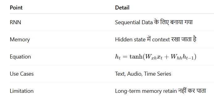
(RNN की संरचना और गणितीय कार्यविधि):अब हम RNN की आंतरिक संरचना (Structure) को विस्तार से समझते हैं — ताकि यह स्पष्ट हो सके कि RNN किस तरह sequential data को process करता है और memory बनाए रखता है।
🔶 1. Basic Idea Behind RNN
RNN का मुख्य विचार यह है कि यह input sequence के हर step पर एक ही cell (या unit) को बार-बार उपयोग करता है, लेकिन हर बार अलग hidden state के साथ।
Structure (Unrolled):
x₁ ──► [RNN Cell] ──► h₁
x₂ ──► [RNN Cell] ──► h₂
x₃ ──► [RNN Cell] ──► h₃
     (shares weights)
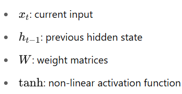
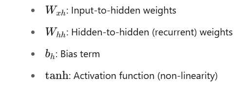
- xt: Input at time step t
- ht: Hidden state at time step t
RNN में hidden state ht, पहले state ht−1 और वर्तमान input xtपर निर्भर करता है।
🧠 2. Key Components of RNN
| Component | Description |
|---|---|
| Input xt | Sequence का current step |
| Hidden state ht | Memory representation |
| Weights W | Shared across time steps |
| Output yt | Final prediction (optional at each step) |
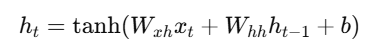
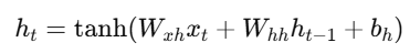
🧮 3. Mathematical Equations
🔹 Hidden State Update:
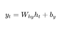
- 🔹 Output (Optional):
🔄 4. Weight Sharing
RNNs में हर time step पर same weights
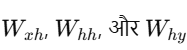
use होते हैं। यह मॉडल को बहुत parameter efficient बनाता है।
🧱 5. RNN Cell Diagram
          x_t
           ↓
      [ Linear Layer ]
           ↓
      + h_{t-1}
           ↓
      [ tanh Activation ]
           ↓
          h_t
           ↓
       (optional)
          y_t
🔧 6. PyTorch Implementation (Simple RNN Layer)
import torch
import torch.nn as nn

rnn = nn.RNN(input_size=8, hidden_size=16, batch_first=True)

x = torch.randn(4, 10, 8)  # batch of 4, sequence length 10, features=8
h0 = torch.zeros(1, 4, 16) # (num_layers, batch, hidden_size)

output, hn = rnn(x, h0)

print(output.shape)  # → [4, 10, 16]
print(hn.shape)      # → [1, 4, 16]
📊 7. Variants of RNNs (आगे के टॉपिक्स)
| Variant | Special Feature |
|---|---|
| Vanilla RNN | Simple structure (as above) |
| LSTM | Long memory, gating mechanism |
| GRU | Efficient, fewer gates than LSTM |
📝 Practice Questions:
- RNN में hidden state क्या दर्शाता है?
- RNN में weight sharing का क्या लाभ है?
- RNN Cell किस तरह input और पिछले state से output निकालता है?
- Mathematical formula for hth_tht क्या है?
- PyTorch में RNN के लिए input tensor का shape क्या होता है?
🎯 Summary
| Concept | Meaning |
|---|---|
| RNN Cell | Basic unit that processes each time step |
| Hidden State | Information summary till time t |
| Shared Weights | Same weights used for all time steps |
| Activation | Usually tanh or ReLU |
| Output | Optional at each step or only at the end |