Anand Singh

Hierarchical Clustering एक ऐसा algorithm है जो डेटा को छोटे clusters से शुरू करके धीरे-धीरे उन्हें merge करता है, जिससे एक Tree-like Structure (Dendrogram) बनता है।यह Unsupervised Learning का एक और महत्वपूर्ण algorithm है जो clustering को सभी levels पर hierarchical रूप में करता है:

सोचिए:
पहले व्यक्ति को परिवारों में बांटा गया → फिर परिवार को समाजों में → फिर समाज को राज्यों में।
यही काम करता है Hierarchical Clustering।

---

🔶 Clustering Approaches:

Method	Description
Agglomerative	Bottom-Up: हर point एक cluster से शुरू करता है → फिर merge होते हैं
Divisive	Top-Down: पूरा dataset एक cluster है → फिर split होते हैं

👉 सबसे सामान्य तरीका: Agglomerative Clustering

---

🧠 Algorithm Steps (Agglomerative):

1. हर data point को एक अलग cluster मानो
2. Closest दो clusters को merge करो
3. Distance matrix update करो
4. Step 2 और 3 को तब तक दोहराओ जब तक एक ही cluster न बच जाए

---

🔍 Linkage Criteria (क्लस्टर्स के बीच दूरी कैसे मापें?)

Linkage Type	Definition
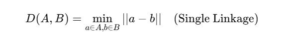
Single	Closest points के बीच की दूरी
Complete	Farthest points के बीच की दूरी
Average	सभी pairwise distances का average
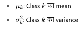
Ward	Variance को minimize करता है (default)

---

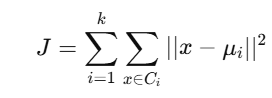
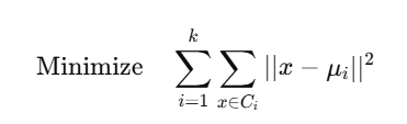
📐 Distance Calculation:

---

✅ Python Code (SciPy + Matplotlib):

import numpy as np
import matplotlib.pyplot as plt
from scipy.cluster.hierarchy import dendrogram, linkage

# Sample Data
X = np.array([[1, 2],
              [2, 3],
              [5, 8],
              [6, 9]])

# Step 1: Linkage matrix
Z = linkage(X, method='ward')

# Step 2: Dendrogram Plot
plt.figure(figsize=(8, 5))
dendrogram(Z, labels=["A", "B", "C", "D"])
plt.title("Hierarchical Clustering Dendrogram")
plt.xlabel("Data Points")
plt.ylabel("Distance")
plt.show()

---

🌲 Dendrogram क्या दर्शाता है?

Dendrogram एक tree diagram होता है जो दिखाता है कि कैसे data points और clusters आपस में जुड़े हुए हैं।

• Y-axis = merging distance
• Horizontal cuts = Desired number of clusters

✂️ अगर आप Y-axis पर एक horizontal लाइन खींचें → आपको अलग-अलग clusters मिलेंगे।

---

🔧 Clustering का निर्माण (sklearn):

from sklearn.cluster import AgglomerativeClustering

model = AgglomerativeClustering(n_clusters=2)
model.fit(X)

print("Cluster Labels:", model.labels_)

---

🔬 Use Cases:

क्षेत्र	उदाहरण
Bioinformatics	Gene expression analysis
Marketing	Customer segmentation
Sociology	Social group formation
Document Analysis	Document/topic clustering

---

⚖️ Pros & Cons:

✅ फायदे:

• कोई need नहीं है k (cluster count) को पहले से जानने की
• Dendrogram से cluster insights आसानी से मिलते हैं
• Complex shape वाले clusters को भी पकड़ सकता है

❌ नुकसान:

• बड़े datasets पर slow होता है
• Distance metrics और linkage method पर भारी निर्भरता
• Non-scalable for huge data

---

📊 Summary Table:

Feature	Hierarchical Clustering
Input	Only Features (No Labels)
Output	Cluster assignments + Dendrogram
Method	Agglomerative / Divisive
Speed	Slow (high computational cost)
Visualization	Dendrogram

---

📝 Practice Questions:

1. Hierarchical Clustering कैसे कार्य करता है?
2. Agglomerative vs Divisive clustering में क्या अंतर है?
3. Linkage criteria में Ward method क्यों उपयोगी है?
4. Dendrogram कैसे interpret किया जाता है?
5. क्या Hierarchical Clustering large datasets के लिए उपयुक्त है?

K-Means Clustering एक Unsupervised Learning Algorithm है जो डेटा को k अलग-अलग clusters में बांटने का कार्य करता है, जहाँ हर cluster में डाले गए डेटा आपस में एक-दूसरे से अधिक समान होते हैं।

उदाहरण:
आप एक दुकान के ग्राहकों को उनके ख़रीदने की आदतों के आधार पर 3 समूहों में बाँटना चाहते हैं — High, Medium, और Low spenders।

---

🔶 उद्देश्य:

K-Means का लक्ष्य है:

Data Points को इस तरह से बांटना कि प्रत्येक Cluster का “Centroid” अपने Points से न्यूनतम दूरी पर हो।

---

📐 Mathematical Objective:

K-Means का Loss Function (Inertia) होता है:

जहाँ:

---

🧠 Algorithm Steps:

1. kkk initial centroids randomly चुनें
2. हर point को सबसे पास वाले centroid के cluster में assign करें
3. हर cluster का नया centroid calculate करें
4. Step 2 और 3 को तब तक दोहराएं जब तक cluster assignment stable ना हो जाए

---

✅ Python Code (with Visualization):

from sklearn.cluster import KMeans
import matplotlib.pyplot as plt
import numpy as np

# Dummy Data
X = np.array([[1, 2], [1, 4], [1, 0],
              [10, 2], [10, 4], [10, 0]])

# KMeans Model
model = KMeans(n_clusters=2, random_state=0)
model.fit(X)

# Output
print("Labels:", model.labels_)                  # Cluster assignments
print("Centroids:", model.cluster_centers_)      # Cluster centers

# Visualization
plt.scatter(X[:, 0], X[:, 1], c=model.labels_, cmap='viridis')
plt.scatter(model.cluster_centers_[:, 0], model.cluster_centers_[:, 1], 
            c='red', marker='X', s=200, label='Centroids')
plt.title("K-Means Clustering")
plt.xlabel("Feature 1")
plt.ylabel("Feature 2")
plt.legend()
plt.grid(True)
plt.show()

---

🔬 Elbow Method (Best k कैसे चुनें?)

Elbow Method यह देखने में मदद करता है कि कितने clusters लेने से सबसे अच्छी grouping मिलेगी।

📈 Plot Inertia vs k:

inertia = []
K = range(1, 10)

for k in K:
    km = KMeans(n_clusters=k)
    km.fit(X)
    inertia.append(km.inertia_)

plt.plot(K, inertia, marker='o')
plt.xlabel('Number of Clusters k')
plt.ylabel('Inertia (Within Sum of Squares)')
plt.title('Elbow Method for Optimal k')
plt.show()

जहाँ graph में “elbow” बनता है — वही optimal k होता है।

---

🔎 Real Life Applications:

Domain	Application Example
Marketing	Customer Segmentation
Healthcare	Disease pattern clustering
Finance	Risk Grouping / Fraud Detection
E-commerce	Product Recommendation (user grouping)

---

⚖️ K-Means के फायदे और नुकसान:

✅ फायदे:

• Simple और Fast
• High-dimensional data पर काम करता है
• Easily scalable

❌ नुकसान:

• kkk पहले से पता होना चाहिए
• Non-spherical clusters को handle नहीं कर पाता
• Outliers पर sensitive होता है
• Local minima में फँस सकता है (initial centroid पर निर्भरता)

---

📊 Summary Table:

Feature	K-Means
Type	Unsupervised Clustering
Input	Only Features (No Labels)
Output	Cluster IDs
Distance Metric	Euclidean Distance (Mostly)
Speed	Fast
Shape Assumption	Spherical Clusters

---

📝 Practice Questions:

1. K-Means का उद्देश्य क्या होता है?
2. Loss function J का अर्थ क्या है?
3. Elbow Method का क्या उपयोग है?
4. K-Means कब खराब perform करता है?
5. K-Means clustering में initialization क्यों महत्वपूर्ण होता है?

Unsupervised Learning वह तकनीक है जहाँ हमें केवल input data दिया जाता है, लेकिन उसके साथ कोई label या output नहीं होता।

Model को खुद से patterns, structure, clusters या associations को सीखना होता है।

---

🧠 उपयोग की परिस्थितियाँ:

Supervised Learning	Unsupervised Learning
X (input) + Y (label)	केवल X (input)
Spam Detection, Price Prediction	Customer Segmentation, Anomaly Detection

---

🔑 उद्देश्य:

Unsupervised Learning का मुख्य उद्देश्य है:

• Hidden patterns खोजना
• Similar data points को एक साथ ग्रुप करना
• Dimensionality को घटाना
• Outlier या anomaly detect करना

---

🔬 प्रमुख Algorithms:

Algorithm	उद्देश्य	उदाहरण
K-Means Clustering	Similarity के आधार पर group बनाना	Customer Segmentation
Hierarchical Clustering	Tree structure में grouping	Genetic Analysis
DBSCAN	Density-based clustering	Outlier Detection
PCA (Principal Component Analysis)	Dimensionality Reduction	Image Compression
Autoencoders	Feature Compression (DL-based)	Anomaly Detection
t-SNE / UMAP	Visualization (2D mapping)	Data Plotting

---

🔷 1. K-Means Clustering

🎯 उद्देश्य:

डाटा को k समूहों (clusters) में बाँटना, जहाँ हर group का center “centroid” होता है।

📐 Mathematical Objective:

जहाँ:

---

✅ Python Code (Sklearn):

from sklearn.cluster import KMeans
import matplotlib.pyplot as plt

X = [[1,2], [1,4], [1,0], [10,2], [10,4], [10,0]]
model = KMeans(n_clusters=2)
model.fit(X)

print(model.labels_)     # Cluster IDs
print(model.cluster_centers_)

plt.scatter(*zip(*X), c=model.labels_)
plt.scatter(*zip(*model.cluster_centers_), c='red', marker='x')
plt.title("K-Means Clustering")
plt.show()

---

🔷 2. Hierarchical Clustering

📌 विशेषताएँ:

• Agglomerative: Bottom-up approach
• Dendrogram के रूप में output मिलता है

✅ Code (SciPy):

from scipy.cluster.hierarchy import dendrogram, linkage
import matplotlib.pyplot as plt

X = [[1,2], [2,3], [10,12], [11,14]]
Z = linkage(X, method='ward')

dendrogram(Z)
plt.title("Hierarchical Clustering Dendrogram")
plt.show()

---

🔷 3. DBSCAN (Density-Based Spatial Clustering)

📌 लाभ:

• Arbitrary shape के clusters बना सकता है
• Outliers को अलग कर सकता है

---

🔷 4. PCA (Principal Component Analysis)

📌 उद्देश्य:

High-dimensional data को कम dimensions में प्रोजेक्ट करना।

📐 PCA Formula:

Data matrix X को transform करते हैं: Z=XW

जहाँ:

• W: Principal components (eigenvectors of covariance matrix)
• Z: Reduced dimensional representation

---

✅ PCA Code:

from sklearn.decomposition import PCA
from sklearn.datasets import load_iris
import matplotlib.pyplot as plt

iris = load_iris()
X = iris.data
pca = PCA(n_components=2)
X_reduced = pca.fit_transform(X)

plt.scatter(X_reduced[:,0], X_reduced[:,1], c=iris.target)
plt.title("PCA of Iris Dataset")
plt.show()

---

📊 Summary Table:

Algorithm	उद्देश्य	Output	Visualization
K-Means	Clustering	Cluster Labels	✅
Hierarchical	Clustering Tree (Dendrogram)	Cluster Tree	✅
DBSCAN	Density-Based Clustering	Labels + Outliers	✅
PCA	Dimension Reduction	Compressed Data	✅
Autoencoders	Neural Compression	Encoded Data	❌ (Complex)

---

📝 Practice Questions:

1. Unsupervised Learning में labels क्यों नहीं होते?
2. K-Means का objective function क्या है?
3. PCA कैसे dimension को reduce करता है?
4. DBSCAN और K-Means में क्या अंतर है?
5. Hierarchical Clustering में Dendrogram क्या दर्शाता है?

Naive Bayes एक probability-based classification algorithm है जो Bayes’ Theorem पर आधारित है।
यह विशेष रूप से text classification (जैसे spam detection, sentiment analysis) में बहुत उपयोगी होता है।

---

🔶 Naive Bayes का मूल सिद्धांत:

इसका आधार है Bayes’ Theorem, जो किसी घटना की posterior probability निकालने के लिए prior probability और likelihood का उपयोग करता है।

📐 Bayes’ Theorem:

जहाँ:

• P(C∣X): Class C की probability दी गई input X के लिए
• P(X∣C): Class C में X के आने की संभावना
• P(C): Class C की prior probability
• P(X): Input X की total probability

---

🎯 Naive Assumption:

Naive Bayes “naive” इस कारण कहलाता है क्योंकि यह मान लेता है कि:

सभी features एक-दूसरे से स्वतंत्र (independent) हैं, यानी

---

🔍 Types of Naive Bayes:

Type	Use Case	Feature Type
Gaussian Naive Bayes	Continuous values (e.g., height)	Numerical
Multinomial NB	Text classification (e.g., spam)	Discrete counts
Bernoulli NB	Binary features (yes/no)	Boolean

---

🔬 Gaussian Naive Bayes Formula:

यदि कोई feature xxx continuous है, तो हम मानते हैं कि वह Gaussian distribution को follow करता है:

जहाँ

---

🔧 Sklearn में Naive Bayes Code:

from sklearn.naive_bayes import GaussianNB

model = GaussianNB()
model.fit(X_train, y_train)

y_pred = model.predict(X_test)

---

📄 Text Classification (Multinomial Naive Bayes) Example:

from sklearn.feature_extraction.text import CountVectorizer
from sklearn.naive_bayes import MultinomialNB

texts = ["spam offer now", "buy cheap", "hello friend", "how are you"]
labels = [1, 1, 0, 0]  # 1=spam, 0=ham

vectorizer = CountVectorizer()
X = vectorizer.fit_transform(texts)

model = MultinomialNB()
model.fit(X, labels)

test = vectorizer.transform(["cheap offer"])
print(model.predict(test))  # Output: [1]

---

📌 Advantages:

✅ Fast और memory-efficient
✅ Probabilistic interpretation (confidence level मिलता है)
✅ Text और NLP tasks में अच्छा काम करता है
✅ कम data पर भी अच्छा perform करता है

---

⚠️ Limitations:

❌ Independence assumption हमेशा सही नहीं होती
❌ Complex datasets में Accuracy कम हो सकती है
❌ Continuous features पर Gaussian assumption जरूरी होता है

---

📊 Summary Table:

Element	Description
Based On	Bayes’ Theorem
Assumption	Feature Independence
Output	Probabilities (0 to 1)
Applications	Spam Detection, NLP, Document Classify
Speed	Very Fast

---

📝 Practice Questions:

1. Naive Bayes का “naive” नाम क्यों पड़ा?
2. Bayes’ Theorem का formula क्या है और उसका अर्थ समझाइए।
3. Gaussian Naive Bayes में likelihood कैसे निकाला जाता है?
4. Multinomial और Bernoulli Naive Bayes में क्या अंतर है?
5. Naive Bayes को कब उपयोग नहीं करना चाहिए?

---

SVM (Support Vector Machine) एक शक्तिशाली classification algorithm है जो high-dimensional spaces में भी शानदार performance देता है।

यह algorithm कोशिश करता है कि classes के बीच सबसे चौड़ा margin (boundary) बने।

---

🔶 क्या है SVM?

SVM एक ऐसा मॉडल है जो अलग-अलग class के data points के बीच सबसे best decision boundary (hyperplane) बनाता है।

🎯 उद्देश्य:

Class 0 और Class 1 को इस तरह से अलग करना कि उनके बीच का फासला (margin) अधिकतम हो।

---

📊 उदाहरण:

Data Point	Feature 1	Feature 2	Class
A	2	3	0
B	4	5	1
C	3	4	0

SVM इसे इस तरह से classify करता है कि class boundaries के पास के points (Support Vectors) अधिकतम दूर हों।

---

🧠 महत्वपूर्ण Concepts:

Term	Meaning
Hyperplane	Decision boundary जो classes को अलग करता है
Margin	Hyperplane से सबसे नजदीक के points तक की दूरी
Support Vectors	वही points जो margin को define करते हैं
Kernel Trick	Non-linear data को linear बनाने की तकनीक

---

🔄 Linear vs Non-Linear SVM:

Type	Use Case
Linear SVM	जब data साफ़-साफ़ linearly separable हो
Non-Linear SVM	जब data का pattern complex हो — इसे kernels से solve करते हैं (RBF, Polynomial etc.)

---

🔧 Scikit-learn में SVM का Implementation:

✅ Linear SVM (with linearly separable data):

from sklearn.svm import SVC

model = SVC(kernel='linear')
model.fit(X_train, y_train)

y_pred = model.predict(X_test)

---

✅ Non-Linear SVM (with RBF Kernel):

model = SVC(kernel='rbf')  # Gaussian kernel
model.fit(X_train, y_train)

---

🔬 Kernel Functions:

Kernel	Description
Linear	Straight line boundary
Polynomial	Polynomial-based curved boundary
RBF (Gaussian)	Smooth, flexible boundary for complex data
Sigmoid	Similar to neural network activation

---

📊 SVM vs अन्य Algorithms:

Feature	SVM	Decision Tree	Logistic Regression
Works in High Dim	✅ Yes	❌ No	❌ No
Handles Non-linearity	✅ via kernel	✅ with tuning	❌ Not naturally
Explainability	❌ Difficult	✅ Yes	✅ Yes
Overfitting	❌ Less prone	✅ More prone	✅ Moderate

---

✅ Visualization (2D Example with Python)

rom sklearn import datasets
from sklearn.svm import SVC
import matplotlib.pyplot as plt
import numpy as np

# Load dummy data
X, y = datasets.make_blobs(n_samples=100, centers=2, random_state=6)

# Train SVM
clf = SVC(kernel='linear')
clf.fit(X, y)

# Plot
plt.scatter(X[:, 0], X[:, 1], c=y)
ax = plt.gca()

# Plot decision boundary
xlim = ax.get_xlim()
ylim = ax.get_ylim()
xx = np.linspace(xlim[0], xlim[1])
yy = np.linspace(ylim[0], ylim[1])
YY, XX = np.meshgrid(yy, xx)
xy = np.vstack([XX.ravel(), YY.ravel()]).T
Z = clf.decision_function(xy).reshape(XX.shape)
ax.contour(XX, YY, Z, levels=[-1, 0, 1], linestyles=['--', '-', '--'])
plt.title("SVM Decision Boundary")
plt.show()

---

📌 कब उपयोग करें SVM?

✅ जब:

• Feature dimension बहुत ज़्यादा हो
• Classes के बीच separation जरूरी हो
• Small dataset हो लेकिन complex pattern हो

---

📝 Practice Questions:

1. SVM का मुख्य उद्देश्य क्या होता है?
2. Support Vectors क्या होते हैं और उनका क्या role है?
3. Kernel trick कैसे काम करती है?
4. Linear और Non-linear SVM में क्या अंतर है?
5. Decision Tree और SVM में क्या अंतर है?