ROC-AUC Curve

जब हम binary classification करते हैं (जैसे spam/not-spam, disease/healthy), तो हमें सिर्फ accuracy से model की गुणवत्ता नहीं पता चलती। ऐसे में ROC-AUC Curve model के prediction scores को analyze करने में मदद करता है।


🔶 ROC का अर्थ:

ROC = Receiver Operating Characteristic
यह एक graphical plot है जो बताता है कि model कैसे विभिन्न thresholds पर perform करता है।

📈 ROC Curve Plot:

  • X-axis → False Positive Rate (FPR)
  • Y-axis → True Positive Rate (TPR)

Threshold को 0 से 1 तक vary करते हुए हम विभिन्न FPR और TPR को plot करते हैं — और वो बनाता है ROC curve.


📐 Formulae:

✅ True Positive Rate (TPR) aka Recall:

✅ False Positive Rate (FPR):
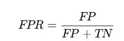

🔷 AUC का अर्थ:

AUC = Area Under the Curve
यह ROC curve के नीचे आने वाले क्षेत्र का मान है।
AUC का मान 0 और 1 के बीच होता है:

AUC ScoreMeaning
1.0Perfect model
0.9 – 1.0Excellent
0.8 – 0.9Good
0.7 – 0.8Fair
0.5Random guess (no skill)
< 0.5Worse than random (bad model)

✅ Python Code (Scikit-learn + Visualization):

from sklearn.datasets import make_classification
from sklearn.linear_model import LogisticRegression
from sklearn.metrics import roc_curve, auc
import matplotlib.pyplot as plt

# Sample data
X, y = make_classification(n_samples=1000, n_classes=2, n_informative=3)

# Train model
model = LogisticRegression()
model.fit(X, y)

# Get predicted probabilities
y_scores = model.predict_proba(X)[:, 1]

# Compute FPR, TPR
fpr, tpr, thresholds = roc_curve(y, y_scores)

# Compute AUC
roc_auc = auc(fpr, tpr)

# Plot
plt.figure(figsize=(8,6))
plt.plot(fpr, tpr, label=f'ROC Curve (AUC = {roc_auc:.2f})')
plt.plot([0, 1], [0, 1], 'k--', label='Random Guess')
plt.xlabel('False Positive Rate')
plt.ylabel('True Positive Rate')
plt.title('ROC-AUC Curve')
plt.legend()
plt.grid(True)
plt.show()

📊 ROC vs Precision-Recall Curve:


Title Page Separator Site title

FeatureROC CurvePrecision-Recall Curve
Focuses onAll classes (balanced data)Positive class (imbalanced data)
X-axisFalse Positive RateRecall
Y-axisTrue Positive Rate (Recall)Precision

✅ Imbalanced datasets पर Precision-Recall Curve ज़्यादा informative हो सकता है।


📄 Summary Table:

ConceptDescription
ROC CurveTPR vs FPR plot for various thresholds
AUCROC Curve के नीचे का क्षेत्र
Best CaseAUC = 1.0 (Perfect classifier)
Worst CaseAUC = 0.5 (Random guessing)
Use CasesBinary classification performance check

📝 Practice Questions:

  1. ROC Curve में X और Y axes क्या दर्शाते हैं?
  2. AUC का score किस range में होता है और उसका क्या मतलब है?
  3. ROC और Precision-Recall Curve में क्या अंतर है?
  4. ROC curve कैसे बनता है?
  5. क्या AUC metric imbalanced datasets के लिए reliable है?

Agent, Environment, Reward

Reinforcement Learning (RL) में एक एजेंट को एक वातावरण (Environment) में रखा जाता है।
वो किसी स्थिति (State) में होता है, वहाँ से एक Action लेता है, और बदले में उसे Reward मिलता है।

सोचिए एक रोबोट का, जो maze से बाहर निकलने की कोशिश कर रहा है — उसे सही रास्ता सीखने के लिए कई बार try करना होगा।


🔑 Key Concepts:

Termअर्थ (Meaning)
Agentवह learner या decision-maker जो actions लेता है
Environmentबाहरी दुनिया जिससे agent interact करता है
State (S)उस समय की स्थिति जहाँ agent है
Action (A)agent द्वारा उठाया गया कदम या फैसला
Reward (R)किसी action पर environment द्वारा दिया गया feedback
Policy (π)Agent का strategy, जो बताती है किस state में कौनसा action लेना है
Value (V)किसी स्थिति में मिलने वाले भविष्य के rewards का अनुमान
Episodeशुरू से लेकर एक goal तक का पूरा sequence

🔄 Agent-Environment Loop:

यह एक continuous feedback loop होता है:

(State s_t) --[action a_t]--> (Environment) --[Reward r_t, next state s_{t+1}]--> (Agent)

Diagram:

+-----------+        action a_t         +-------------+
| | -----------------------> | |
| AGENT | | ENVIRONMENT |
| | <----------------------- | |
+-----------+ r_t, s_{t+1} +-------------+

🧠 उद्देश्य:

Agent का लक्ष्य होता है:

Maximum cumulative reward (return) प्राप्त करना

Return:

जहाँ

  • γ: Discount Factor (0 < γ ≤ 1)
  • Future rewards की importance को नियंत्रित करता है

🎮 उदाहरण:

ProblemAgentEnvironmentReward
गेम खेलना (e.g. Chess)Chess AIChess boardजीतने पर +1, हारने पर -1
Self-driving carCar controllerसड़क और ट्रैफिकटकराने पर -ve, सही चलने पर +ve
Robo-navigationRobotMaze/GridExit मिलने पर +10

🧮 Formal Definition (Markov Decision Process – MDP):

Reinforcement Learning को formal रूप में एक MDP से दर्शाया जा सकता है: MDP=(S,A,P,R,γ)

जहाँ:

  • S: States का सेट
  • A: Actions का सेट
  • P: Transition probabilities
  • R: Reward function
  • γ: Discount factor

✅ Python Code Example (Gym Environment):

import gym

# Environment
env = gym.make("CartPole-v1")
state = env.reset()

for _ in range(10):
env.render()
action = env.action_space.sample() # Random action
next_state, reward, done, info = env.step(action)
print("Reward:", reward)
if done:
break

env.close()

🎯 Summary Table:

TermDescription
AgentDecision-maker (e.g., robot, AI model)
EnvironmentExternal system (e.g., game, world)
StateCurrent situation or context
ActionAgent का निर्णय या प्रयास
Rewardपर्यावरण का response, जो सीखने में मदद करता
Policyनियम जो बताता है क्या करना है
GoalTotal reward को maximize करना

📝 Practice Questions:

  1. Reinforcement Learning में Agent और Environment क्या भूमिका निभाते हैं?
  2. Reward और Return में क्या अंतर है?
  3. Discount factor (γ\gammaγ) क्या है और इसका महत्व क्या है?
  4. RL में Policy और Value function का क्या कार्य होता है?
  5. कोई real-life उदाहरण दीजिए जहाँ RL model प्रयोग हो सकता है।

Deep Learning in Real-World Applications

अब हम Deep Learning के Real World Applications को देखेंगे — जहाँ ये तकनीक सच में ज़िंदगी बदल रही है।

🤖 “AI अब सिर्फ लैब की चीज़ नहीं – ये हमारे चारों ओर है!”


🔷 1. Overview

Deep Learning आज लगभग हर industry में क्रांति ला चुका है। इसकी self-learning, pattern recognition, और prediction power की वजह से इसे healthcare, finance, robotics, media, agriculture, हर क्षेत्र में adopt किया जा रहा है।


🔶 2. Major Application Areas

✅ A. Computer Vision

ApplicationUse Case Example
Face RecognitionFace Unlock, CCTV Surveillance
Object DetectionSelf-driving cars, Security systems
Medical ImagingTumor detection from MRI/CT
OCRHandwritten → Digital text
Image CaptioningDescribing scenes (blind assistance)

✅ B. Natural Language Processing (NLP)

ApplicationUse Case Example
Machine TranslationGoogle Translate, Meta AI Translate
Sentiment AnalysisBrand reputation, customer feedback
Chatbots & AssistantsAlexa, ChatGPT, Siri, Google Assistant
Text SummarizationNews, Legal Docs, Academic papers
Language ModelingCode completion, Writing assistants

✅ C. Healthcare

ApplicationUse Case Example
Disease DiagnosisDiabetic Retinopathy, Skin Cancer
Medical ImagingTumor detection, Radiology assistance
Drug DiscoveryProtein structure prediction (AlphaFold)
Personalized TreatmentRisk profiling, survival prediction

✅ D. Finance

ApplicationUse Case Example
Fraud DetectionAnomaly spotting in transactions
Stock Market PredictionDeep learning-based forecasting
Credit ScoringRisk profiling using neural networks
Algorithmic TradingReal-time buy/sell decisions

✅ E. Autonomous Systems

ApplicationUse Case Example
Self-Driving CarsTesla Autopilot, Waymo, Cruise
DronesObject following, Aerial delivery
RoboticsPicking, sorting, warehouse automation

✅ F. Recommendation Systems

ApplicationUse Case Example
Movie RecommendationsNetflix, Prime Video
E-commerceAmazon product suggestions
Music & PodcastsSpotify, YouTube Music

✅ G. Generative AI

ApplicationUse Case Example
Text-to-ImageDALL·E, Stable Diffusion
Image-to-ImageColorization, Super-Resolution
Deepfake GenerationSynthetic media
Text GenerationChatGPT, Copywriting bots
Code GenerationGitHub Copilot, Replit Ghostwriter

🔷 3. Success Stories

CompanyApplicationImpact
GoogleBERT, AlphaFold, ImagenNLP & Biology breakthrough
TeslaVision + Planning AISelf-driving
OpenAIGPT, DALL·ELanguage & Creativity
MetaLLaMA, Segment AnythingVision + Language
NVIDIADL for GPU optimizationAI hardware + DL synergy

🔶 4. Future of Deep Learning

✅ General-purpose agents
✅ AI + Robotics + Language = Real World AI
✅ Biology + Deep Learning = Protein, Genetics
✅ AI for Climate, Agriculture, Education
✅ Personalized tutors, doctors, coaches


📝 Practice Questions:

  1. Computer Vision में deep learning के 3 practical uses बताइए।
  2. Healthcare में AI diagnosis कैसे मदद करता है?
  3. NLP के किन real-world applications में deep learning का उपयोग हो रहा है?
  4. Recommendation system में DL का रोल क्या है?
  5. Generative AI और deep learning कैसे जुड़े हैं?

🔚 Summary

DomainExample Use Case
VisionFace detection, Cancer scans
LanguageChatGPT, Translation, Summarization
FinanceFraud detection, Trading bots
HealthcareMedical imaging, Drug discovery
AutomationSelf-driving, Drones
GenerativeText → Image, Code generation

Explainable AI (XAI)

अब हम एक बहुत ज़रूरी और व्यावहारिक विषय को समझते हैं — जिसका मक़सद है AI को “क्यों” और “कैसे” समझाना

🧠 “AI का फ़ैसला समझ में आना चाहिए – काला जादू नहीं।”


🔷 1. What is Explainable AI?

Explainable AI (XAI) का उद्देश्य है कि AI/ML models के निर्णय साफ़, पारदर्शी और इंसानों के समझने लायक हों।

“Why did the model predict this?”
“What part of the input influenced the decision?”


🔶 2. Why XAI is Important?

कारणउदाहरण
✅ TrustDoctor को explainable model चाहिए
✅ DebuggingDeveloper model की गलती पकड़ सकता है
✅ FairnessBias या discrimination detect हो सकता है
✅ RegulationGDPR / Medical AI में जरूरी है

🔷 3. Black Box vs Explainable Models

Model TypeExplainability
Linear Regression✅ High
Decision Trees✅ Medium
Deep Neural Nets❌ Low (Black box)
Transformers, CNN❌ Complex

इसलिए हमें DNN, CNN, Transformers जैसे models के लिए XAI techniques चाहिए।


🔶 4. Popular XAI Techniques

✅ A. Feature Importance (Tabular data)

  • Tree-based models (like Random Forests) naturally बताते हैं कि कौन-सा feature कितना important है.

✅ B. LIME (Local Interpretable Model-Agnostic Explanations)

Model की prediction के आसपास एक simple interpretable model fit किया जाता है।

pip install lime
from lime.lime_tabular import LimeTabularExplainer

✅ C. SHAP (SHapley Additive exPlanations)

Game Theory आधारित: हर feature की contribution value निकाली जाती है।

pip install shap
import shap
explainer = shap.Explainer(model.predict, X_test)
shap_values = explainer(X_test[:10])
shap.plots.waterfall(shap_values[0])

✅ D. Saliency Maps (Image models)

CNN model के output को किस image region ने प्रभावित किया?

# torch.autograd + image gradient → heatmap

✅ E. Grad-CAM (CNN explainability)

किसी image में कौन-से हिस्से ने prediction को सबसे ज़्यादा influence किया?

pip install grad-cam
  • Input image → CNN → last conv layer → gradients → visualization map

✅ F. Attention Visualization (Transformer models)

Transformer models (like BERT, GPT) में Attention Score से पता चलता है कि model ने किस word पर सबसे ज़्यादा ध्यान दिया।

from transformers import BertTokenizer, BertModel
# Visualize attention weights

🔷 5. Real-World Applications

DomainExplanation Use
HealthcareDoctor को पता चले AI ने क्या देखा
FinanceLoan rejection के कारण समझाना
Legalकिसी भी decision का कारण trace करना
Autonomous CarsSensor input के आधार पर फ़ैसला क्यों लिया गया?

🔶 6. Challenges in XAI

समस्याकारण
Complex modelsMillions of parameters
No ground truthक्या explanation सही है?
Trade-offExplainability vs Accuracy

🧠 Summary

AspectDescription
XAI क्या हैAI को explain करना इंसानों के लिए
क्यों ज़रूरीTrust, Regulation, Debugging
TechniquesLIME, SHAP, Grad-CAM, Attention
Domain UseMedical, Finance, Legal, Vision

📝 Practice Questions:

  1. Explainable AI की ज़रूरत क्यों है?
  2. LIME और SHAP में क्या अंतर है?
  3. CNN models को explain करने के लिए कौन-सी technique use होती है?
  4. Grad-CAM क्या है और कैसे काम करता है?
  5. XAI healthcare में कैसे मदद करता है?

Diffusion Models

अब हम deep learning की सबसे आधुनिक और प्रभावशाली तकनीकों में से एक को सीखने जा रहे हैं — जो text-to-image जैसे tasks में breakthroughs लाई है:

🔍 धीरे-धीरे noise जोड़ो, फिर धीरे-धीरे उसे हटाकर नया data generate करो!


🔷 1. What are Diffusion Models?

Diffusion Models एक तरह के generative models हैं, जो training में images में noise डालते हैं और फिर सीखते हैं उसे वापस original image में बदलना।

🧠 Goal: Noise से high-quality image generate करना।


🔶 2. Real World Analogy

कल्पना कीजिए आपके पास एक साफ़ तस्वीर है, जिसे आप बार-बार थोड़ा-थोड़ा धुंधला (noise) करते हैं। अब model सीखता है कि कैसे इस धुंधली तस्वीर से साफ़ तस्वीर वापस बनाई जाए।


🔷 3. Core Idea

Diffusion Process में दो चरण होते हैं:

✅ 1. Forward Process (Adding Noise)

Original image में step-by-step Gaussian noise मिलाया जाता है।

  • जहां x_0 = original image
  • x_t = noisy image at step t
  • ε = Gaussian noise

✅ 2. Reverse Process (Denoising)

Model सीखता है कि इस noise को step-by-step हटाकर original image कैसे reconstruct की जाए।


🔶 4. Intuition:

Stageक्या हो रहा है
Forward ProcessImage → Noise
Reverse ProcessNoise → Image (generate करने के लिए!)

🔷 5. Architecture

Diffusion models आमतौर पर U-Net architecture का उपयोग करते हैं।

  • Noise-added image input किया जाता है
  • Time-step embedding दिया जाता है
  • U-Net output करता है predicted noise
  • Loss: MSE between actual noise और predicted noise

🔶 6. Training Objective

Model को सिखाया जाता है:

यानी: Model सिखे कि original noise (ε) क्या था, ताकि उसे हटाकर साफ़ image बन सके।


🔷 7. Famous Diffusion Models

ModelHighlightsOrganization
DDPMDenoising Diffusion Probabilistic ModelGoogle
Stable DiffusionText-to-Image diffusion modelStability AI
ImagenHigh-quality generation from textGoogle Brain
DALLE-2CLIP + DiffusionOpenAI

🔶 8. Applications of Diffusion Models

✅ Text-to-Image Generation
✅ Inpainting (Missing image fill करना)
✅ Super-resolution
✅ Audio synthesis
✅ 3D scene generation


🔷 9. Sample Code (Simplified PyTorch)

import torch
import torch.nn as nn

class SimpleDenoiseModel(nn.Module):
def __init__(self):
super().__init__()
self.net = nn.Sequential(
nn.Linear(784, 512),
nn.ReLU(),
nn.Linear(512, 784),
)
def forward(self, x, t):
return self.net(x)

# Forward diffusion (add noise)
def add_noise(x, t):
noise = torch.randn_like(x)
alpha = 1 - 0.02 * t # Simplified
return alpha * x + (1 - alpha) * noise, noise

🧠 Difference from GANs

FeatureGANDiffusion Model
Stable❌ Hard to train✅ More stable
Output QualityMedium to High✅ High
Mode Collapse❌ Possible✅ Rare
Training TimeFaster❌ Slower
Use CaseImage, video, textMostly high-fidelity images

📝 Practice Questions:

  1. Diffusion model में forward और reverse process क्या होते हैं?
  2. Stable Diffusion किस technique पर आधारित है?
  3. GAN और Diffusion में क्या अंतर है?
  4. Time-step embedding क्यों ज़रूरी है?
  5. Diffusion से कौन-कौन से real-world tasks solve किए जा सकते हैं?

🧾 Summary

ConceptDescription
Forward PassClean image → Add noise
Reverse PassNoisy image → Remove noise (generate)
ArchitectureMostly U-Net
Training LossMSE between true and predicted noise
OutputNew image generated from pure noise