Backpropagation and Training ,Forward Pass and Loss Calculation

(बैकप्रोपेगेशन और प्रशिक्षण प्रक्रिया)


🔷 1. Introduction (परिचय)

Backpropagation = “Backwards propagation of errors”
यह एक algorithm है जो Neural Network के weights को loss function के आधार पर update करता है।


🔁 2. Training का पूरा Flow

  1. Forward Pass:
    Input → Hidden → Output
    (Prediction generate होता है)
  2. Loss Calculation:
    Prediction और Ground Truth के बीच Loss मापा जाता है
  3. Backward Pass (Backpropagation):
    Loss का Gradient calculate होता है हर weight के लिए
  4. Weight Update (Optimizer):
    Gradient Descent द्वारा Weights को update किया जाता है
  5. Repeat for Epochs:
    जब तक model सटीक prediction न करने लगे

🔧 3. Backpropagation: कैसे काम करता है?

Backpropagation एक mathematical tool है जो Chain Rule of Calculus का उपयोग करता है:

जहाँ:

  • L: Loss
  • y: Prediction
  • z: Neuron input
  • w: Weight

🧠 Visual Diagram (Flowchart):

Input → Hidden → Output → Loss

Backpropagate Gradient

Update Weights (via Optimizer)

💻 PyTorch में Training Code (Simple)

import torch
import torch.nn as nn
import torch.optim as optim

# Simple Model
model = nn.Linear(1, 1)
criterion = nn.MSELoss()
optimizer = optim.SGD(model.parameters(), lr=0.01)

# Training Data
x = torch.tensor([[1.0], [2.0]])
y = torch.tensor([[2.0], [4.0]])

# Training Loop
for epoch in range(10):
outputs = model(x) # Forward
loss = criterion(outputs, y) # Compute Loss

optimizer.zero_grad() # Clear gradients
loss.backward() # Backpropagation
optimizer.step() # Update weights

print(f"Epoch {epoch+1}, Loss: {loss.item():.4f}")

🔍 Important Terms Recap

TermExplanation
Forward PassPrediction बनाना
Lossगलती मापना
Backward PassGradient निकालना
OptimizerWeight update करना
EpochDataset पर एक complete pass

🎯 Learning Objectives Summary

  • Backpropagation सीखने का आधार है
  • यह Loss function के gradient के आधार पर weights को सुधारता है
  • Optimizer gradient का उपयोग कर model को बेहतर बनाता है
  • पूरा training loop PyTorch में automate होता है

📝 अभ्यास प्रश्न (Practice Questions)

  1. Backpropagation किस rule पर आधारित है?
  2. Forward Pass और Backward Pass में क्या अंतर है?
  3. Loss.backward() क्या करता है?
  4. Optimizer.zero_grad() क्यों ज़रूरी है?
  5. एक training loop के चार मुख्य steps क्या होते हैं?

Forward Pass and Loss Calculation

(फ़ॉरवर्ड पास और लॉस की गणना)

🔶 1. Forward Pass (इनपुट से आउपट तक की यात्रा)

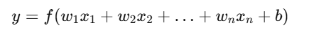
Forward Pass वह चरण है जिसमें neural network किसी इनपुट को लेकर उसे विभिन्न layers के माध्यम से प्रवाहित करता है ताकि अंतिम output (prediction) उत्पन्न हो।

🔁 Step-by-Step Process:

  1. Input Vector (x) network में भेजा जाता है
  2. Each Layer:
    • Performs a linear transformation

Applies an activation function

  1. Final output layer देता है prediction y^

🧠 Neural Network Flow:

scssCopyEditInput → Hidden Layer 1 → Hidden Layer 2 → ... → Output Layer → Prediction
  • Linear + Activation sequence हर layer पर लागू होता है
  • Output layer की activation function task पर निर्भर करती है (जैसे classification के लिए softmax या sigmoid)

📌 Forward Pass का उद्देश्य:

  • Input features को progressively abstract करना
  • Neural network के current weights से output generate करना
  • इस output को असली label से compare कर पाने लायक बनाना

🔷 2. Loss Calculation (Prediction की ग़लती मापना)

Once prediction (y^​) is ready, it is compared to the true label (y) using a Loss Function.
Loss function हमें बताता है prediction कितना सही या गलत है।


🔢 Common Loss Functions:


🔁 Loss Calculation का Flow:

  1. Prediction (y^​) compute करो
  2. Ground truth label yसे compare करो
  3. Error calculate करो using loss function
  4. यही error backpropagation में propagate किया जाएगा

💻 PyTorch Example: Loss and Prediction

import torch
import torch.nn as nn

# Input and True label
x = torch.tensor([[1.0, 2.0]])
y_true = torch.tensor([[0.0]])

# Define simple model
model = nn.Sequential(
nn.Linear(2, 3),
nn.ReLU(),
nn.Linear(3, 1),
nn.Sigmoid()
)

# Loss function
criterion = nn.BCELoss()

# Forward Pass
y_pred = model(x)

# Loss Calculation
loss = criterion(y_pred, y_true)

print("Prediction:", y_pred.item())
print("Loss:", loss.item())

🔁 Complete Diagram Flow:

Input → Hidden → Output → Loss

Backpropagate Gradient

Update Weights (via Optimizer)

✅ यह दर्शाता है कि forward pass prediction करता है, और loss function उस prediction की गुणवत्ता को मापता है।


📌 Summary Table

StepDescription
Forward PassInput को through layers भेजना
OutputPrediction generate करना
Loss CalculationPrediction और label के बीच का अंतर मापना
Next StepLoss को use करके gradient calculate करना

🎯 Objectives Recap:

  • Forward Pass transforms input → prediction
  • Loss function tells how wrong the prediction is
  • Loss is key for guiding weight updates

📝 Practice Questions:

  1. Forward Pass में कौन-कौन सी operations होती हैं?
  2. z=Wx+b का क्या अर्थ है?
  3. Binary Classification के लिए कौन-सा loss function उपयोग होता है?
  4. Loss function और optimizer में क्या अंतर है?
  5. PyTorch में loss calculate करने के लिए कौन-कौन सी steps होती हैं?

Loss Functions and Optimization

(हानि फलन और अनुकूलन विधियाँ)


🔷 1. Loss Function (हानि फलन) क्या है?

Loss function यह मापता है कि आपके मॉडल की prediction असली output से कितनी दूर है।

🔁 Role in Training:

  • Prediction → Loss Function → Error → Backpropagation → Weight Update

📌 कार्य:

Stepकार्य
PredictionOutput generate करना
Lossगलती मापना
BackpropagationGradient निकालना
OptimizerWeights update करना

🔹 2. Loss Function के प्रकार

🔸 A. Regression Problems के लिए:

✅ Mean Squared Error (MSE):

  • Continuous values के लिए
  • Output को penalize करता है अगर prediction और label का अंतर बड़ा हो

✅ Mean Absolute Error (MAE):

  • Outliers से कम प्रभावित

🔸 B. Classification Problems के लिए:

✅ Binary Cross Entropy:

L=−[ylog⁡(p)+(1−y)log⁡(1−p)]

  • Binary classification के लिए
  • Sigmoid + BCELoss

✅ Categorical Cross Entropy:

  • Multi-class classification
  • Softmax + CrossEntropyLoss

💻 PyTorch Examples:

import torch
import torch.nn as nn

# MSE Loss
mse_loss = nn.MSELoss()
pred = torch.tensor([2.5])
target = torch.tensor([3.0])
print("MSE:", mse_loss(pred, target).item())

# Binary Cross Entropy
bce_loss = nn.BCELoss()
pred = torch.tensor([0.9])
target = torch.tensor([1.0])
print("BCE:", bce_loss(pred, target).item())

🔧 3. Optimization (अनुकूलन)

Optimizer वह algorithm है जो model के weights को loss minimize करने के लिए update करता है।


🔸 4. Common Optimization Algorithms

OptimizerDescription
SGDSimple gradient descent
MomentumAdds momentum to SGD updates
RMSPropAdaptive learning rate, good for RNN
AdamAdaptive + Momentum = Most widely used

🔁 Gradient Descent Update Rule:

जहाँ:

  • η: Learning rate
  • ∂L/∂w: Gradient of loss w.r.t. weights

⚠️ Learning Rate की भूमिका:

Learning Rateपरिणाम
बहुत छोटाSlow training
बहुत बड़ाOvershooting, unstable
सहीFast & stable convergence

💻 PyTorch में Optimizer:

import torch.optim as optim

model = torch.nn.Linear(1, 1)
optimizer = optim.Adam(model.parameters(), lr=0.01)

# Example training step:
loss = torch.tensor(0.5, requires_grad=True)
loss.backward()
optimizer.step()
optimizer.zero_grad()

🎯 Objectives Summary

  • Loss function prediction error को मापता है
  • Optimizers gradients का उपयोग कर weights को update करते हैं
  • PyTorch में loss + optimizer combo सबसे जरूरी सेटअप है

📝 अभ्यास प्रश्न (Practice Questions)

  1. Loss Function और Optimizer में क्या अंतर है?
  2. MSE और MAE में क्या अंतर है?
  3. Binary Cross-Entropy का फॉर्मूला लिखिए
  4. Adam Optimizer कैसे काम करता है?
  5. नीचे दिए गए कोड का output क्या होगा?

loss = torch.tensor(1.0, requires_grad=True) loss.backward() print(loss.grad)

Activation Functions

(सक्रियण फलन: Sigmoid, Tanh, ReLU)


🔷 1. परिचय (Introduction)

Neural Network में Activation Function यह तय करता है कि कोई neuron “active” होगा या नहीं।
यह non-linearity लाता है, ताकि मॉडल complex patterns को सीख सके।


🔹 2. आवश्यकता क्यों? (Why Needed?)

बिना Activation Function के neural network एक simple linear model बन जाएगा।

📌 With Activation Function → Deep, non-linear models
📌 Without Activation → सिर्फ linear transformation


🔶 3. मुख्य Activation Functions


🔸 A. Sigmoid Function

📌 Output Range: (0, 1)
📌 उपयोग: Binary classification, Logistic regression

✅ लाभ:

  • Probability की तरह आउटपुट देता है
  • Smooth gradient

❌ कमी:

  • Gradient vanishing problem
  • Output range छोटा है

📈 ग्राफ: S-shaped (S-curve)


🔸 B. Tanh (Hyperbolic Tangent)

📌 Output Range: (-1, 1)
📌 उपयोग: जब input data zero-centered हो

✅ लाभ:

  • Stronger gradients than sigmoid
  • Centered at 0 → better learning

❌ कमी:

  • Still suffers from vanishing gradient (large input पर gradient → 0)

📈 ग्राफ: S-shaped but centered at 0


🔸 C. ReLU (Rectified Linear Unit)

📌 Output Range: [0, ∞)
📌 उपयोग: Deep Networks में सबसे आम activation

✅ लाभ:

  • Fast computation
  • Sparse activation (only positive values pass)
  • No vanishing gradient for positive inputs

❌ कमी:

  • Dying ReLU Problem: negative input → always zero gradient

📈 ग्राफ: 0 for x < 0, linear for x > 0


🔁 तुलना तालिका (Comparison Table)

FeatureSigmoidTanhReLU
Output Range(0, 1)(-1, 1)[0, ∞)
Non-linearity
Vanishing GradientYesYesNo (partial)
SpeedSlowSlowFast
UsageBinary outputsHidden layers (earlier)Deep models (most common)

💻 PyTorch Code: Activation Functions

import torch
import torch.nn.functional as F

x = torch.tensor([-2.0, 0.0, 2.0])

print("Sigmoid:", torch.sigmoid(x))
print("Tanh:", torch.tanh(x))
print("ReLU:", F.relu(x))

🎯 Learning Summary (सारांश)

  • Sigmoid और Tanh smooth functions हैं लेकिन saturation (vanishing gradient) से ग्रस्त हो सकते हैं
  • ReLU simple, fast, और deep networks में सबसे अधिक उपयोगी है
  • Hidden layers में ReLU सबसे लोकप्रिय choice है

📝 अभ्यास प्रश्न (Practice Questions)

  1. Sigmoid और Tanh में क्या अंतर है?
  2. ReLU का गणितीय फॉर्मूला क्या है?
  3. Dying ReLU problem क्या है?
  4. यदि input -3 हो तो ReLU का output क्या होगा?
  5. नीचे दिए गए PyTorch कोड का आउटपुट बताइए:

x = torch.tensor([-1.0, 0.0, 1.0]) print(torch.tanh(x))

Perceptron and Multi-layer Perceptron (MLP)

(परसेप्ट्रॉन और मल्टी-लेयर परसेप्ट्रॉन)


🔷 1. Perceptron: Single-layer Neural Unit

➤ परिभाषा:

Perceptron एक single-layer feedforward neural network है जो binary classification करने में सक्षम होता है।

🧮 गणितीय रूप:


📌 विशेषताएँ:

गुणविवरण
Structureएक ही layer (input से output)
UseLinear binary classification
LimitationNon-linear problems (जैसे XOR) solve नहीं कर सकता

🔁 Simple Diagram:


🔶 2. MLP: Multi-layer Perceptron

➤ परिभाषा:

MLP एक feedforward artificial neural network है जिसमें एक या अधिक hidden layers होते हैं।

🏗️ संरचना:

Input → Hidden Layer(s) → Output
(हर layer में neurons होते हैं, और हर neuron activation function apply करता है)


📌 विशेषताएँ:

गुणविवरण
Structure2+ layers (input, hidden, output)
UseComplex, non-linear problems
TrainingBackpropagation + Gradient Descent
ActivationReLU, sigmoid, tanh, softmax

🔁 MLP Diagram (Structure):


💻 PyTorch में एक सरल MLP कोड:

import torch.nn as nn

class MLP(nn.Module):
def __init__(self):
super(MLP, self).__init__()
self.net = nn.Sequential(
nn.Linear(3, 5), # Input layer → Hidden
nn.ReLU(),
nn.Linear(5, 1), # Hidden → Output
nn.Sigmoid()
)

def forward(self, x):
return self.net(x)

🔄 तुलना तालिका: Perceptron vs MLP

विशेषताPerceptronMLP
LayersSingleMultiple (hidden included)
ActivationStep/SigmoidReLU, Sigmoid, Tanh, Softmax
Data Handlingकेवल linearly separableComplex, non-linear data
LearningSimple weight updateBackpropagation algorithm

🎯 Learning Summary:

  • Perceptron एक सबसे सरल Neural Network है।
  • MLP में Hidden layers होने से यह complex pattern सीख सकता है।
  • Deep Learning में MLP सबसे बुनियादी और आधारभूत संरचना है।

📝 अभ्यास प्रश्न (Practice Questions):

  1. Perceptron का गणितीय फ़ॉर्मूला क्या है?
  2. Perceptron और MLP में मुख्य अंतर क्या है?
  3. MLP में activation functions क्यों ज़रूरी होते हैं?
  4. Perceptron XOR problem क्यों solve नहीं कर सकता?
  5. एक सरल MLP में कितनी layers होती हैं?

Biological Neuron vs Artificial Neuron

(जैविक न्यूरॉन बनाम कृत्रिम न्यूरॉन)


🔹 1. Biological Neuron (जैविक न्यूरॉन) क्या होता है?

यह मानव मस्तिष्क की मूल इकाई है जो संकेतों (signals) को लेती है, प्रक्रिया करती है और अन्य न्यूरॉनों को भेजती है।

🔬 संरचना (Structure):

भागकार्य
DendritesInput signal लेते हैं
Cell Body (Soma)Input को process करता है
AxonOutput signal को भेजता है
Synapseदो neurons के बीच signal पास करता है

🧠 कार्यप्रणाली:

  • जब कुल Input signal एक Threshold से ऊपर जाता है, तब neuron “Fire” करता है (Signal भेजता है)।

🔹 2. Artificial Neuron (कृत्रिम न्यूरॉन)

Deep Learning में Artificial Neuron का उपयोग किया जाता है, जो Biological neuron से प्रेरित है लेकिन गणितीय होता है।

🔢 कार्यप्रणाली:

  • xi​: Inputs
  • wi: Weights
  • b: Bias
  • f: Activation function
  • y: Output

🔁 तुलनात्मक तालिका (Comparison Table)

विशेषताजैविक न्यूरॉनकृत्रिम न्यूरॉन
संरचनाDendrites, Axon, SynapseInputs, Weights, Activation
संकेत (Signal)ElectrochemicalNumerical (वास्तविक संख्या)
प्रसंस्करणThreshold based firingWeighted sum + Activation
सीखनाSynapse के बदलाव सेWeights update (Gradient Descent)
नेटवर्कBiological Neural NetworkArtificial Neural Network (ANN)

🧠 विज़ुअल तुलना (Diagram)

Biological Neuron:                        Artificial Neuron:

Input (Dendrites) x1, x2, x3 →
↓ ↓
Cell Body (Summation) w1x1 + w2x2 + w3x3 + b
↓ ↓
Axon → Output Activation Function → Output

🔍 निष्कर्ष (Conclusion):

  • Artificial Neurons inspired हैं Biological Neurons से, परंतु वे सरल गणितीय मॉडल हैं।
  • एक Artificial Neuron सिर्फ एक छोटा सा भाग है Deep Learning नेटवर्क का, लेकिन उसका inspiration मानव मस्तिष्क से आया है।
  • जैसा मानव मस्तिष्क सिखता है अनुभव से, वैसे ही ANN सिखता है डेटा से।

🎯 उद्देश्य (Objective Summary)

  • जैविक न्यूरॉन की संरचना और कार्यप्रणाली समझना
  • कृत्रिम न्यूरॉन का गणितीय स्वरूप जानना
  • दोनों के बीच की समानता और भिन्नता पहचानना
  • Deep Learning में इस संबंध का महत्व समझना

📝 अभ्यास प्रश्न (Practice Questions)

  1. Dendrites और Axon का कार्य क्या होता है?
  2. Artificial Neuron किस प्रकार का Input लेता है?
  3. दोनों प्रकार के न्यूरॉन में signal कैसा होता है?
  4. एक Artificial Neuron का गणितीय formula लिखिए।
  5. कृत्रिम न्यूरॉन जैविक न्यूरॉन से कैसे प्रेरित है?