ML

क्या आपको पता है कि Machine Learning Engineers इस समय में सबसे ज़्यादा paid tech professionals हैं?

इनकी average salary लगभग £100k है — जो software engineers, AI engineers, और data scientists से भी ज़्यादा है।

लेकिन ध्यान दें दोस्तों, बात सिर्फ़ salary की नहीं है।

एक Machine Learning Engineer के तौर पर आपको मिलती है:

• Fascinating problems को हल करने का मौका
• Cutting-edge tools के साथ प्रयोग करने का अवसर
• दुनिया पर positive impact डालने की satisfaction

तो इस article में, मैं आपको एक clear और simple learning roadmap दूँगा जिससे आप Machine Learning Engineer बन सकते हैं। साथ ही, मैं आपको best resources भी बताऊँगा।

चलिए शुरू करते हैं! 🚀

---

🧮 Maths और Statistics

मैंने ये बात कई बार कही है — लेकिन अगर आप Machine Learning या पूरे Data Field में करियर बनाना चाहते हैं,
तो Maths और Statistics सबसे ज़्यादा ज़रूरी चीज़ें हैं जो आपको सीखनी चाहिए।

Technologies आती-जाती रहती हैं — जैसे Blockchain या AI,
लेकिन Mathematics सदियों से एक मूल आधार (fundamental staple) बना हुआ है।

अच्छी बात ये है कि आपको Maths Genius होने की ज़रूरत नहीं है।
मैं अपने first-hand experience से कह सकता हूँ कि Machine Learning में काम करने के लिए बस उतनी ही maths चाहिए
जितनी आपको school के आखिरी सालों या undergraduate STEM degree के पहले-दूसरे साल में सिखाई जाती है।

---

📘 3 Main Areas of Focus

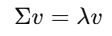
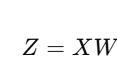
1. Linear Algebra (रेखीय बीजगणित) →
   इसमें आप matrices, eigenvalues, vectors जैसी चीज़ें सीखते हैं।
   ये concepts हर जगह इस्तेमाल होते हैं — जैसे Principal Component Analysis (PCA), TensorFlow,
   यहाँ तक कि एक dataframe भी एक तरह की matrix ही होती है।
2. Calculus (कलन) →
   इससे आप differentiation सीखते हैं — यानी कैसे gradient descent और backpropagation algorithms अंदर से काम करते हैं।
   ये हर machine learning algorithm के training और learning process में उपयोग होते हैं।
3. Statistics (सांख्यिकी) →
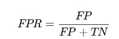
   इसमें आप सीखेंगे: probability, distributions, Bayesian statistics, Central Limit Theorem, और Maximum Likelihood Estimation
   इन तीनों में से Statistics सबसे ज़्यादा valuable है। अगर आप शुरुआत कर रहे हैं, तो अपना ज़्यादातर ध्यान Statistics पर ही दें।

---

🐍 Python

Python को Machine Learning की मुख्य भाषा माना जाता है —
कई beginners और मेरे coaching clients में मैंने देखा कि लोग हमेशा “best Python course” ढूँढते रहते हैं।

मैं दोहराऊँगा – “best” जैसा कुछ नहीं होता।
कोई भी popular Python introduction course चलेगा क्योंकि सब में लगभग वही concepts सिखाए जाते हैं।

---

🔑 Python Basics

• Native Data Structures → dict, tuple, list
• Loops → for और while
• Conditional Statements → if-else
• Functions और Classes
• Common Libraries
• Design Patterns

---

🧠 Python Packages for ML

• NumPy → Arrays के लिए numerical computing
• Pandas → Data manipulation और analysis
• Matplotlib → Data visualization और plotting
• Scikit-learn → Fundamental ML algorithms implement करने के लिए
• SciPy → General scientific computing के लिए

---

📚 Python Resources

1. W3Schools Python Course
2. Python for Everybody Specialisation
3. Machine Learning with Python and Scikit-Learn 

---

🧩 SQL

एक Machine Learning Engineer के लिए SQL भी बहुत जरूरी है।
खासकर जब आप datasets बनाते हैं या feature engineering करते हैं।

मैं अपने अनुभव से कह सकता हूँ कि मैं लगभग 30–40% समय SQL में बिताता हूँ।
यानी ये बहुत ज़रूरी skill है।

---

📘 SQL Topics to Learn

• SELECT * FROM, AS
• ALTER, INSERT, CREATE, UPDATE, DELETE
• GROUP BY, ORDER BY
• WHERE, AND, OR, BETWEEN, IN, HAVING
• AVG, COUNT, MIN, MAX, SUM
• FULL JOIN, LEFT JOIN, RIGHT JOIN, INNER JOIN, UNION
• CASE, IFF
• DATEADD, DATEDIFF, DATEPART
• PARTITION BY, QUALIFY, ROW()

---

📚 SQL Resources

1. The Complete SQL Bootcamp: Go from Zero to Hero
2. W3Schools SQL Tutorial
3. TutorialsPoint SQL Tutorial

Free resources काफी हैं, इसलिए course खरीदने की ज़रूरत नहीं।
और अगर कहीं अटक जाएँ, तो ChatGPT हमेशा मदद कर सकता है। 💡

---

🤖 Machine Learning

Machine Learning Engineer बनने के लिए ML algorithms सीखना बेहद जरूरी है।
ये roadmap का fun part है और ज्यादातर लोग इसी कारण इस field में आते हैं।

सच कहूँ तो, इन algorithms को सीखना हमेशा fun नहीं होता।
थोड़ा mental effort और समय लगता है, लेकिन धीरे-धीरे सब समझ में आ जाएगा और मेहनत worth it होगी।

---

🔑 Key Algorithms और Concepts

• Linear, Logistic और Polynomial Regression
• Generalised Linear Models (GLM) और Generalised Additive Models (GAM)
• Decision Trees, Random Forests, Gradient-Boosted Trees
• Support Vector Machines (SVM)
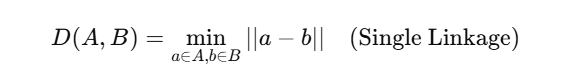
• K-Means और K-Nearest Neighbour Clustering
• Feature Engineering (categorical features)
• Evaluation Metrics
• Regularisation, Bias vs Variance Tradeoff, Cross-Validation
• Gradient Descent और Backpropagation

---

📚 ML Resources

1. Machine Learning Specialisation by Andrew Ng → Best starter course
2. The Hundred-Page ML Book → Concise और practical
3. Hands-On ML with Scikit-Learn, Keras, and TensorFlow → Entry/mid-level ML engineers के लिए complete guide

---

🧠 Deep Learning

Fundamental ML algorithms ही career में सबसे ज़्यादा काम आते हैं।
लेकिन Deep Learning important है:

• NLP (Natural Language Processing)
• Computer Vision

Areas to Study

• Neural Networks → ML की foundation
• Convolutional Neural Networks (CNNs) → Image detection
• Recurrent Neural Networks (RNNs) → Time series और NLP
• Transformers → Current state-of-the-art

Resources

• Deep Learning Specialization by Andrew Ng
• Neural Networks: Zero to Hero (YouTube) → Andrej Karpathy
• Deep Learning (Adaptive Computation and ML series) → Yoshua Bengio

---

🛠 Software Engineering

Machine Learning Engineer बनने के लिए software engineering fundamentals जानना जरूरी है।

Areas

1. Data Structures & Algorithms → Arrays, Linked Lists, Queues, Sorting, Binary Search, Trees, Hashing, Graphs
2. System Design → Networking, APIs, Caching, Proxies, Storage
3. Production Code → Typing, Linting, Testing, DRY, KISS, YAGNI
4. APIs → ML models को API endpoints के रूप में serve करना

---

☁️ MLOps

Jupyter Notebook में model का business value नहीं है।
आपको deploy करना सीखना होगा।

Learn

• Cloud → AWS, GCP, Azure
• Containerisation → Docker, Kubernetes
• Version Control → Git, GitHub
• Shell/Terminal →

PCA (Principal Component Analysis) एक statistical technique है जो high-dimensional data को कम dimensions में project करके उसका meaningful structure retain करती है।

उदाहरण के लिए:
अगर आपके पास 100 features हैं, लेकिन असल में केवल 2 features पूरे pattern को explain कर सकते हैं — तो PCA उन्हीं 2 को चुनता है।

---

🔶 उद्देश्य:

• Features की संख्या को घटाना (Dimensionality Reduction)
• Data में मौजूद variance को अधिकतम बनाए रखना
• Visualization को आसान बनाना
• Noise को घटाना और Model को Fast बनाना

---

📐 Core Idea (Mathematical):

PCA का लक्ष्य होता है:

ऐसे नए axes (Principal Components) खोजना जो original data में सबसे अधिक variance को capture करें।

🎯 Objective:

जहाँ:

• X: Centered data matrix
• W: Projection matrix (eigenvectors)
• Z: Projected data (principal components)

---

🧮 Step-by-Step Working:

Standardize the Data
(mean = 0, std = 1)

Covariance Matrix Calculate करो

Eigenvalues और Eigenvectors निकालो

Top-k Eigenvectors को चुनो (सबसे बड़ी eigenvalues वाले)

Data को Project करो new space में:

---

✅ Python Code (Sklearn + Visualization):

from sklearn.decomposition import PCA
from sklearn.datasets import load_iris
import matplotlib.pyplot as plt

# Load sample data
data = load_iris()
X = data.data
y = data.target

# PCA with 2 components
pca = PCA(n_components=2)
X_pca = pca.fit_transform(X)

# Plot
plt.figure(figsize=(8,6))
plt.scatter(X_pca[:,0], X_pca[:,1], c=y, cmap='viridis')
plt.xlabel("Principal Component 1")
plt.ylabel("Principal Component 2")
plt.title("PCA: Iris Dataset")
plt.grid(True)
plt.show()

---

📊 Explained Variance:

PCA बताता है कि हर component कितना information retain करता है:

print(pca.explained_variance_ratio_)

उदाहरण Output:

[0.9246, 0.0530] → यानी कुल 97.76% variance केवल 2 components से explain हो गया

---

🔎 कब इस्तेमाल करें PCA?

Case	उपयोग
बहुत सारे features हों	✅
Model slow या overfit कर रहा हो	✅
Feature correlation ज़्यादा हो	✅
Features sparse हों (जैसे TF-IDF)	✅

---

⚠️ Limitations:

Limitation	Explanation
Interpretability कम हो जाती है	PCs original features से अलग होते हैं
केवल linear patterns detect करता है	Complex nonlinear pattern नहीं देख सकता
Scaling आवश्यक है	बिना scaling result गलत हो सकता है

---

📊 Summary Table:

Feature	PCA
Type	Dimensionality Reduction
Preserves	Maximum Variance
Based On	Eigenvalues & Eigenvectors
Suitable For	High-dimensional, numeric data
Output	Reduced dimension components

---

📝 Practice Questions:

1. PCA का उद्देश्य क्या होता है?
2. Covariance matrix किस लिए बनाई जाती है?
3. Eigenvectors और Eigenvalues का क्या अर्थ है PCA में?
4. Explained Variance Ratio क्या दर्शाता है?
5. PCA कब काम नहीं करता?

Hierarchical Clustering एक ऐसा algorithm है जो डेटा को छोटे clusters से शुरू करके धीरे-धीरे उन्हें merge करता है, जिससे एक Tree-like Structure (Dendrogram) बनता है।यह Unsupervised Learning का एक और महत्वपूर्ण algorithm है जो clustering को सभी levels पर hierarchical रूप में करता है:

सोचिए:
पहले व्यक्ति को परिवारों में बांटा गया → फिर परिवार को समाजों में → फिर समाज को राज्यों में।
यही काम करता है Hierarchical Clustering।

---

🔶 Clustering Approaches:

Method	Description
Agglomerative	Bottom-Up: हर point एक cluster से शुरू करता है → फिर merge होते हैं
Divisive	Top-Down: पूरा dataset एक cluster है → फिर split होते हैं

👉 सबसे सामान्य तरीका: Agglomerative Clustering

---

🧠 Algorithm Steps (Agglomerative):

1. हर data point को एक अलग cluster मानो
2. Closest दो clusters को merge करो
3. Distance matrix update करो
4. Step 2 और 3 को तब तक दोहराओ जब तक एक ही cluster न बच जाए

---

🔍 Linkage Criteria (क्लस्टर्स के बीच दूरी कैसे मापें?)

Linkage Type	Definition
Single	Closest points के बीच की दूरी
Complete	Farthest points के बीच की दूरी
Average	सभी pairwise distances का average
Ward	Variance को minimize करता है (default)

---

📐 Distance Calculation:

---

✅ Python Code (SciPy + Matplotlib):

import numpy as np
import matplotlib.pyplot as plt
from scipy.cluster.hierarchy import dendrogram, linkage

# Sample Data
X = np.array([[1, 2],
              [2, 3],
              [5, 8],
              [6, 9]])

# Step 1: Linkage matrix
Z = linkage(X, method='ward')

# Step 2: Dendrogram Plot
plt.figure(figsize=(8, 5))
dendrogram(Z, labels=["A", "B", "C", "D"])
plt.title("Hierarchical Clustering Dendrogram")
plt.xlabel("Data Points")
plt.ylabel("Distance")
plt.show()

---

🌲 Dendrogram क्या दर्शाता है?

Dendrogram एक tree diagram होता है जो दिखाता है कि कैसे data points और clusters आपस में जुड़े हुए हैं।

• Y-axis = merging distance
• Horizontal cuts = Desired number of clusters

✂️ अगर आप Y-axis पर एक horizontal लाइन खींचें → आपको अलग-अलग clusters मिलेंगे।

---

🔧 Clustering का निर्माण (sklearn):

from sklearn.cluster import AgglomerativeClustering

model = AgglomerativeClustering(n_clusters=2)
model.fit(X)

print("Cluster Labels:", model.labels_)

---

🔬 Use Cases:

क्षेत्र	उदाहरण
Bioinformatics	Gene expression analysis
Marketing	Customer segmentation
Sociology	Social group formation
Document Analysis	Document/topic clustering

---

⚖️ Pros & Cons:

✅ फायदे:

• कोई need नहीं है k (cluster count) को पहले से जानने की
• Dendrogram से cluster insights आसानी से मिलते हैं
• Complex shape वाले clusters को भी पकड़ सकता है

❌ नुकसान:

• बड़े datasets पर slow होता है
• Distance metrics और linkage method पर भारी निर्भरता
• Non-scalable for huge data

---

📊 Summary Table:

Feature	Hierarchical Clustering
Input	Only Features (No Labels)
Output	Cluster assignments + Dendrogram
Method	Agglomerative / Divisive
Speed	Slow (high computational cost)
Visualization	Dendrogram

---

📝 Practice Questions:

1. Hierarchical Clustering कैसे कार्य करता है?
2. Agglomerative vs Divisive clustering में क्या अंतर है?
3. Linkage criteria में Ward method क्यों उपयोगी है?
4. Dendrogram कैसे interpret किया जाता है?
5. क्या Hierarchical Clustering large datasets के लिए उपयुक्त है?