ML Archives - Page 12 of 17

Sequence Data and Time-Series

July 11, 2025 by Anand Singh

(क्रमिक डेटा और समय-श्रृंखला)

🔶 1. Sequence Data क्या होता है?

📌 परिभाषा:

Sequence Data ऐसा data होता है जिसमें values का क्रम (order) मायने रखता है।
हर एक input पिछले inputs पर निर्भर हो सकता है।

📍 Examples:

एक वाक्य के शब्द (sentence)
संगीत के सुर
मौसम के data में तापमान
किसी ग्राहक का खरीद इतिहास

🔁 “Sequence” का अर्थ है — ordered और dependent items.

🔶 2. Time-Series Data क्या होता है?

📌 परिभाषा:

Time-Series एक special type का sequence data है जिसमें observations समय के अनुसार क्रमबद्ध होते हैं।

📍 Examples:

Stock prices per day/hour
Temperature per minute
Website traffic per week
Electricity usage per second

🔁 इसमें समय (time stamp) बहुत ही महत्वपूर्ण होता है।

📊 3. Sequence vs Time-Series: Difference

Feature	Sequence Data	Time-Series Data
Order	Important	Important
Time Interval	Optional	Must be fixed or known
Examples	Text, DNA, events	Temperature, stock, traffic
Goal	Next item prediction, labeling	Forecasting, anomaly detection

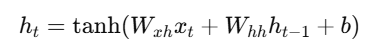
🧠 4. Why RNN is Good for Sequence/Time-Series?

RNN एक ऐसा neural network है जो past context को memory में रखता है और next output को प्रभावित करता है।

✅ It remembers
✅ It learns from history
✅ It handles variable-length input

🔄 5. Use Cases of Sequence and Time-Series with RNNs:

Use Case	Description
Language Modeling	Next word prediction
Sentiment Analysis	Text को classify करना
Stock Price Prediction	Future price estimation
Weather Forecasting	Future temperature/humidity
Machine Translation	Sequence to sequence conversion
Activity Detection	Sensor-based human activity detection

🔧 6. PyTorch Example: RNN for Time-Series Input

import torch
import torch.nn as nn

rnn = nn.RNN(input_size=1, hidden_size=20, num_layers=1, batch_first=True)

# Input: batch of 5 samples, each with 10 timesteps, each step has 1 feature
input = torch.randn(5, 10, 1)
h0 = torch.zeros(1, 5, 20)

output, hn = rnn(input, h0)
print(output.shape)  # → [5, 10, 20]

🔁 7. Time-Series Forecasting Flow:

Past Inputs (x₁, x₂, ..., xₜ)  
       ↓
   RNN Model  
       ↓
Predicted Output (xₜ₊₁)

Optionally: Use sliding window for training

Example: Use past 10 days’ stock prices to predict the 11th

📈 8. Time-Series Challenges:

Challenge	Description
Trend	Long-term increase or decrease
Seasonality	Repeating patterns (e.g. daily, yearly)
Noise	Random fluctuations
Missing Data	Gaps in time
Non-Stationarity	Changing mean/variance over time

RNNs, LSTMs, and GRUs are commonly used to handle these!

📝 Practice Questions:

Sequence data और time-series data में क्या अंतर है?
Time-series को predict करने के लिए RNN क्यों उपयुक्त है?
Time-series data में कौन-कौन सी समस्याएं आती हैं?
Sliding window क्या होता है?
PyTorch में time-series data को कैसे format करते हैं?

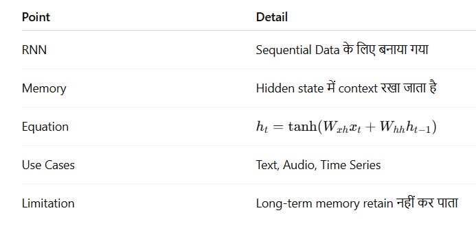
🎯 Summary:

Concept	Explanation
Sequence Data	Ordered, context-dependent data
Time-Series	Temporal, time-dependent data
RNN	Learns from previous steps
Use Cases	Text, sensor, finance, environment
Challenges	Trends, seasonality, missing data

Introduction to RNNs

July 13, 2025July 11, 2025 by Anand Singh

(रीकरेंट न्यूरल नेटवर्क का परिचय)

🔶 1. What is an RNN?

RNN (Recurrent Neural Network) एक ऐसा neural network है जो input के रूप में मिलने वाले sequence data को process करता है, और past inputs की जानकारी को याद रखकर अगले outputs तय करता है।

Simple terms में:
RNNs “memory” रखते हैं और इससे वो time-dependent problems solve कर सकते हैं।

🔁 2. क्यों ज़रूरी है RNN?

Traditional Neural Networks (जैसे MLP या CNN) हर input को independent मानते हैं।

लेकिन sequential data (जैसे भाषा, मौसम का डेटा, stock prices) में ऐसा नहीं होता —
पहले शब्द या डेटा का अगली स्थिति पर प्रभाव होता है।

🧠 RNN इस dependency को capture करने में सक्षम है।

📈 3. Examples of Sequence Tasks:

Application	Input	Output
Sentiment Analysis	Sentence	Sentiment
Machine Translation	Sentence in English	Sentence in Hindi
Speech Recognition	Audio Signal	Text
Time Series Forecasting	Past values	Future value

🧱 4. RNN Architecture:

Basic Structure:

x₁ → [RNN Cell] → h₁  
x₂ → [RNN Cell] → h₂  
x₃ → [RNN Cell] → h₃  
... and so on

हर step पर output ht निर्भर करता है:

जहाँ:

🔁 5. RNN Memory Concept:

RNN में hidden state hth_tht एक प्रकार की memory की तरह काम करता है।
हर नए input के साथ यह update होता है — जिससे model को context याद रहता है।

🔄 6. Unrolling an RNN:

RNN को एक loop में चलाया जाता है, लेकिन हम इसे unroll कर सकते हैं:

x1 → [ ] → h1  
x2 → [ ] → h2  
x3 → [ ] → h3

→ यह loop-based representation है जिसमें एक ही cell बार-बार चलता है।

🔧 7. PyTorch Code: Basic RNN Example

import torch
import torch.nn as nn

rnn = nn.RNN(input_size=10, hidden_size=20, num_layers=1, batch_first=True)

input = torch.randn(5, 3, 10)     # (batch, sequence, input_size)
h0 = torch.zeros(1, 5, 20)        # (num_layers, batch, hidden_size)

output, hn = rnn(input, h0)

print(output.shape)  # → [5, 3, 20]
print(hn.shape)      # → [1, 5, 20]

⚠️ 8. Limitations of Vanilla RNN

Problem	Reason
Vanishing Gradient	Long-term dependencies भूल जाते हैं
Exploding Gradient	Gradient बहुत बढ़ जाता है
Short Memory	केवल कुछ पिछले steps को याद रख पाता है

👉 इसका समाधान है: LSTM और GRU (अगले topics में आएगा)

📘 Summary:

📝 Practice Questions:

RNN किस प्रकार की समस्याओं को हल करने के लिए उपयुक्त है?
Hidden state का क्या काम होता है RNN में?
RNN को unroll करना क्या होता है?
RNN के कौन-कौन से limitations हैं?
PyTorch में एक simple RNN कैसे implement करते हैं?

Famous CNN Architectures (LeNet, AlexNet, VGG, ResNet)

July 11, 2025 by Anand Singh

🔶 1. LeNet-5 (1998) – By Yann LeCun

🕰 वर्ष: 1998
👤 Developer: Yann LeCun, Léon Bottou, Yoshua Bengio, Patrick Haffner

📌 विवरण:

LeNet-5 को Yann LeCun ने विकसित किया था, और इसे पहली बार बैंकिंग सिस्टम में ZIP code पढ़ने के लिए उपयोग किया गया।
यह architecture CNN की पहली वास्तविक success story मानी जाती है।

📚 महत्व:

MNIST जैसे digit recognition datasets पर काफी सफल रहा
पहली बार convolution, pooling, और fully connected layers का इस्तेमाल एक structure में किया गया
यह काम Bell Labs में किया गया था

📌 Use Case: Handwritten digit recognition (MNIST)

🧱 Architecture:

Input: 32x32 Grayscale Image  
→ Conv (6 filters, 5x5)  
→ Avg Pooling  
→ Conv (16 filters, 5x5)  
→ Avg Pooling  
→ Flatten  
→ FC (120)  
→ FC (84)  
→ Output (10 classes)

✅ Highlights:

पहली सफल CNN architecture
बहुत कम parameters
आज भी MNIST जैसे tasks पर उपयोगी

🔶 2. AlexNet (2012) – By Alex Krizhevsky et al.

📌 Use Case: ImageNet Large Scale Visual Recognition Challenge (ILSVRC)

🕰 वर्ष: 2012
👤 Developer: Alex Krizhevsky, Ilya Sutskever, Geoffrey Hinton
🏫 संस्थान: University of Toronto

📌 विवरण:

AlexNet ने 2012 में ImageNet Large Scale Visual Recognition Challenge (ILSVRC) में हिस्सा लिया और बाकी सभी models से बहुत आगे निकल गया — 15.3% error से सीधे 10.1% पर आया।

📚 महत्व:

Deep Learning की mainstream लोकप्रियता इसी model से शुरू हुई
First CNN जिसने GPU का उपयोग करके बहुत बड़ा dataset train किया
Introduced ReLU, Dropout, और Data Augmentation

🧱 Architecture:

Input: 224x224x3 Image  
→ Conv1 (96 filters, 11x11, stride 4)  
→ MaxPool  
→ Conv2 (256 filters, 5x5)  
→ MaxPool  
→ Conv3 (384 filters, 3x3)  
→ Conv4 (384 filters, 3x3)  
→ Conv5 (256 filters, 3x3)  
→ MaxPool  
→ Flatten  
→ FC (4096)  
→ FC (4096)  
→ FC (1000)

✅ Highlights:

ReLU activation introduced
Used Dropout and Data Augmentation
Trained on GPU
Won ILSVRC 2012 with huge margin

🔶 3. VGGNet (2014) – By Oxford (Simonyan & Zisserman)

📌 Use Case: ImageNet Classification

🕰 वर्ष: 2014
👤 विकासकर्ता: Karen Simonyan & Andrew Zisserman
🏫 संस्थान: University of Oxford – Visual Geometry Group (VGG)

📌 विवरण:

VGGNet ने convolution layers को एक uniform pattern (3×3 filters) में रखा, जिससे deeper networks को design करना सरल हो गया।

📚 महत्व:

Depth बढ़ाने से accuracy कैसे improve होती है, यह दिखाया
आज भी कई pre-trained models और transfer learning में उपयोग किया जाता है
VGG-16 और VGG-19 के रूप में दो variants प्रसिद्ध हैं

🧱 Architecture (VGG-16):

Input: 224x224x3  
→ (Conv 3x3, 64) ×2  
→ MaxPool  
→ (Conv 3x3, 128) ×2  
→ MaxPool  
→ (Conv 3x3, 256) ×3  
→ MaxPool  
→ (Conv 3x3, 512) ×3  
→ MaxPool  
→ (Conv 3x3, 512) ×3  
→ MaxPool  
→ Flatten  
→ FC (4096)  
→ FC (4096)  
→ FC (1000)

✅ Highlights:

Simple, uniform design
Uses only 3×3 convolution filters
Very deep (~16–19 layers)
More accurate than AlexNet, but slower

🔶 4. ResNet (2015) – By Microsoft Research

📌 Use Case: Deep classification without degradation

🕰 वर्ष: 2015
👤 विकासकर्ता: Kaiming He, Xiangyu Zhang, Shaoqing Ren, Jian Sun
🏢 संस्थान: Microsoft Research

📌 विवरण:

ResNet ने deep learning की सबसे बड़ी समस्या — Vanishing Gradient — को solve किया, जिससे 100+ layers वाले deep networks train हो सके।

📚 महत्व:

Introduced Residual (Skip) Connections, जिससे deep models भी सीख सकते हैं
2015 ILSVRC में 1st position हासिल की
आज के अधिकांश deep vision models (e.g., Faster R-CNN, Mask R-CNN, ResNeXt) ResNet के foundation पर बने हैं

🧱 Key Innovation: Residual Connections

Output = F(x) + x

🧱 Architecture (ResNet-50):

Uses bottleneck blocks:
- Conv1x1 → Conv3x3 → Conv1x1
- Shortcut connections (skip layers)
Total ~50 layers
Variants: ResNet-18, 34, 50, 101, 152

✅ Highlights:

Solves vanishing gradient problem
Enables very deep networks (100+ layers)
Won ILSVRC 2015

📊 Comparison Table:

Model	Year	Layers	Key Feature	Use Case
LeNet	1998	~7	Simplicity	Digit Recognition
AlexNet	2012	8	ReLU, GPU, Dropout	Large-scale image classification
VGG-16	2014	16	Uniform 3×3 filters	ImageNet
ResNet-50	2015	50	Residual connections	Deep classification

📈 Visual Insight:

LeNet → Basic template
AlexNet → CNN popularized
VGG → Depth with simplicity
ResNet → Deepest with performance

🔧 PyTorch Example: Load Pretrained ResNet

from torchvision import models

model = models.resnet50(pretrained=True)

📝 Practice Questions:

LeNet और AlexNet में क्या अंतर है?
VGG architecture में सभी convolutions का आकार 3×3 क्यों रखा गया?
ResNet में residual connection का क्या लाभ है?
AlexNet को GPU पर क्यों train किया गया था?
ResNet को 100+ layers तक train करना कैसे संभव हो पाया?

🎯 Summary:

Architecture	Best For	Key Contribution
LeNet	Simple tasks	CNN base design
AlexNet	Complex images	ReLU, GPU training
VGG	Clean structure	Deep with uniformity
ResNet	Ultra-deep nets	Skip connections

Use of CNN in Image Classification

July 11, 2025 by Anand Singh

(छवि वर्गीकरण में CNN का उपयोग)

🔶 1. Image Classification क्या है?

📌 परिभाषा:

Image Classification एक ऐसा task है जिसमें input image को एक predefined class में classify किया जाता है।

उदाहरण: एक model को बताना कि image में dog है या cat।

🎯 2. CNN क्यों बेहतर है Image Classification के लिए?

CNN में मौजूद:

Convolution layers → local patterns और textures पहचानती हैं
Pooling layers → size reduce कर feature को concentrate करती हैं
Dense layers → final decision लेती हैं

👉 ये सब मिलकर CNN को image data पर बहुत सक्षम बना देती हैं।

🧠 3. Typical Image Classification Pipeline (Using CNN)

[Input Image]
      ↓
Convolution Layers (Feature Extraction)
      ↓
ReLU + Pooling Layers
      ↓
Flatten Layer
      ↓
Fully Connected (Dense) Layers
      ↓
Softmax (Output → Class Probabilities)

📷 4. Real-world Examples:

Dataset	Classes	Application
MNIST	10 (digits)	Handwritten digit recognition
CIFAR-10	10 (animals, vehicles)	Object classification
ImageNet	1000+	Large-scale classification

🔍 5. Feature Hierarchy in CNN:

Layer Depth	Learns What
Shallow (1-2)	Edges, corners, color blobs
Mid (3-4)	Textures, patterns
Deep (5+)	Objects, faces, full shapes

🔧 6. PyTorch Code Example: CNN for Image Classification (CIFAR-10)

import torch.nn as nn

class CIFAR10CNN(nn.Module):
    def __init__(self):
        super(CIFAR10CNN, self).__init__()
        self.net = nn.Sequential(
            nn.Conv2d(3, 32, 3, padding=1),
            nn.ReLU(),
            nn.MaxPool2d(2, 2),
            nn.Conv2d(32, 64, 3, padding=1),
            nn.ReLU(),
            nn.MaxPool2d(2, 2),
            nn.Flatten(),
            nn.Linear(64 * 8 * 8, 128),
            nn.ReLU(),
            nn.Linear(128, 10)  # 10 output classes for CIFAR-10
        )

    def forward(self, x):
        return self.net(x)

📊 7. Output Layer (Softmax)

nn.Softmax(dim=1)

Converts raw outputs (logits) to probabilities
Highest probability class is the predicted label

📈 8. Training Process (Overview)

Step	Description
Data Preparation	Image resize, normalization
Forward Pass	Prediction
Loss Calculation	CrossEntropyLoss
Backward Pass	Gradients calculate
Optimization	SGD, Adam, etc.
Evaluation	Accuracy, Precision, Recall

✅ 9. Advantages of CNNs in Image Classification

Benefit	Explanation
Local Feature Extraction	Captures spatial hierarchy
Translation Invariance	Position of object doesn’t matter
Parameter Efficiency	Filters shared across image
End-to-End Learning	No need for manual feature extraction

📝 Practice Questions:

CNN image classification में कैसे मदद करता है?
एक simple CNN architecture लिखिए जो 10-class classification कर सके।
Feature map क्या होता है?
CNN में object recognition की hierarchy क्या होती है?
PyTorch में prediction probabilities कैसे निकाली जाती हैं?

🎯 Summary:

Concept	Use in Classification
Convolution	Extract features from images
Pooling	Downsample and focus on important parts
Dense Layers	Final decision making
Softmax	Class probability distribution
CNN	End-to-end feature learning system

CNN Layers (Convolution, Pooling, Flatten, Dense)

July 11, 2025 by Anand Singh

(CNN में Layers कैसे काम करती हैं?)

🔶 1. Overview of CNN Architecture

CNN का उद्देश्य raw images से automatically important features निकालना और उन्हें classification, detection या segmentation के लिए इस्तेमाल करना होता है।

CNN typically निम्नलिखित layers में बँटा होता है:

[Input Image]
   ↓
Convolution Layer
   ↓
Activation (ReLU)
   ↓
Pooling Layer
   ↓
(Repeat Conv + Pool) ...
   ↓
Flatten Layer
   ↓
Dense Layer(s)
   ↓
Output (e.g. Softmax)

🧩 2. Detailed Explanation of Each Layer

✅ A. Convolution Layer

Input image से features extract करता है
Multiple filters apply होते हैं
Output = Feature Maps

Math: y=w∗x+b

PyTorch:

nn.Conv2d(in_channels=3, out_channels=16, kernel_size=3, stride=1, padding=1)

✅ B. Activation Function (ReLU)

Non-linearity introduce करता है
Negative values को 0 कर देता है

f(x)=max⁡(0,x)

PyTorch:

nn.ReLU()

✅ C. Pooling Layer (MaxPooling or AvgPooling)

Feature map को compress करता है
Important features retain करता है
Overfitting reduce करता है

Types:

Max Pooling: Max value select करता है
Average Pooling: Average लेता है

PyTorch:

nn.MaxPool2d(kernel_size=2, stride=2)

✅ D. Flatten Layer

2D feature maps को 1D vector में convert करता है
ताकि Dense Layer उसे process कर सके

Example:

Shape: (Batch, Channels, Height, Width) → (Batch, Features)

PyTorch:

x = x.view(x.size(0), -1)

✅ E. Fully Connected (Dense) Layer

Neural network के traditional layer
Classification या regression करता है

PyTorch:

nn.Linear(in_features=512, out_features=10)

📊 CNN Architecture Diagram (Example)

Input: 32x32x3 (RGB Image)
   ↓
Conv (3x3, 16 filters) → 32x32x16
   ↓
ReLU
   ↓
MaxPool (2x2) → 16x16x16
   ↓
Conv (3x3, 32 filters) → 16x16x32
   ↓
ReLU
   ↓
MaxPool (2x2) → 8x8x32
   ↓
Flatten → 2048
   ↓
Dense → 128
   ↓
Output → 10 classes

🔧 3. PyTorch Code (Simple CNN Model)

import torch.nn as nn

class SimpleCNN(nn.Module):
    def __init__(self):
        super(SimpleCNN, self).__init__()
        self.conv_layers = nn.Sequential(
            nn.Conv2d(3, 16, 3, padding=1),  # Conv1
            nn.ReLU(),
            nn.MaxPool2d(2, 2),             # Pool1
            nn.Conv2d(16, 32, 3, padding=1),# Conv2
            nn.ReLU(),
            nn.MaxPool2d(2, 2)              # Pool2
        )
        self.fc_layers = nn.Sequential(
            nn.Flatten(),
            nn.Linear(32 * 8 * 8, 128),     # Flatten to Dense
            nn.ReLU(),
            nn.Linear(128, 10)              # Output
        )

    def forward(self, x):
        x = self.conv_layers(x)
        x = self.fc_layers(x)
        return x

📈 Summary Table:

Layer	Purpose	Output Shape
Conv	Features extract	(H, W, Filters)
ReLU	Non-linearity	Same as input
Pooling	Downsample	(H/2, W/2, Filters)
Flatten	Vector बनाना	(1D features)
Dense	Predict classes	Output classes

📝 Practice Questions:

Convolution layer में filter क्या करता है?
MaxPooling और AveragePooling में क्या फर्क है?
Flatten क्यों ज़रूरी होता है CNN में?
Dense Layer का काम क्या होता है CNN में?
PyTorch में CNN model define करने का तरीका बताइए।