Decision Trees & Random Forest


🔷 परिचय:

Decision Trees और Random Forest Supervised Learning के दो बहुत लोकप्रिय और शक्तिशाली एल्गोरिद्म हैं।
ये विशेष रूप से तब उपयोगी होते हैं जब हमें explainable और interpretive मॉडल चाहिए होते हैं।

आप सोचिए एक इंसान कैसे फैसला करता है?
अगर “Age > 30” है → फिर “Income > ₹50k” → फिर निर्णय लें
ऐसा ही काम करता है Decision Tree.


🔶 1. Decision Tree (निर्णय वृक्ष)

📌 क्या है?

Decision Tree एक ट्री-आधारित मॉडल है जो डेटा को विभाजित (Split) करता है ताकि decision तक पहुँचा जा सके।

📊 उदाहरण:

              आयु > 30?
/ \
हाँ नहीं
/ \
वेतन > 50k? No
/ \
हाँ नहीं
Yes No

✅ विशेषताएँ:

विशेषताविवरण
Model TypeClassification या Regression
Input DataStructured tabular data
OutputClass label या Continuous value
Splitting BasisGini, Entropy, या MSE
Explainabilityबहुत अच्छी

🛠️ Decision Tree कैसे बनता है?

  1. Dataset के किसी feature पर split करो
  2. Split के बाद Impurity कम होनी चाहिए (Gini या Entropy)
  3. यही recursively करते हुए tree expand होता है
  4. Leaf nodes पर final class या value तय होती है

✅ स्किकिट-लर्न (Scikit-Learn) कोड:

from sklearn.tree import DecisionTreeClassifier

model = DecisionTreeClassifier(criterion='gini') # या entropy
model.fit(X_train, y_train)

y_pred = model.predict(X_test)

🔷 2. Random Forest (रैंडम फॉरेस्ट)

📌 क्या है?

Random Forest एक ensemble learning तकनीक है जो कई Decision Trees को मिलाकर एक मजबूत मॉडल बनाती है।

एक Decision Tree = एक डॉक्टर की राय
Random Forest = 100 डॉक्टरों की राय का औसत
अधिक Trees → बेहतर फैसला


✅ विशेषताएँ:

विशेषताविवरण
Algorithm TypeBagging (Bootstrap Aggregation)
Model StrengthHigh Accuracy, Low Variance
Overfittingकम होता है
Decision MethodVoting (Classification) / Averaging (Regression)

🛠️ कैसे काम करता है?

  1. Dataset से random sampling के कई subsets बनते हैं
  2. हर subset पर एक अलग Decision Tree train होता है
  3. Prediction के समय: सभी trees की राय ली जाती है
  4. Final prediction: Majority Vote या Average

✅ स्किकिट-लर्न कोड:

from sklearn.ensemble import RandomForestClassifier

model = RandomForestClassifier(n_estimators=100, criterion='gini')
model.fit(X_train, y_train)

y_pred = model.predict(X_test)

🔍 Decision Tree vs Random Forest

विशेषताDecision TreeRandom Forest
AccuracyMediumHigh
Overfitting RiskHighLow
ExplainabilityHighLow
SpeedFastSlower (more trees)
Use CasesSimple decision makingHigh performance tasks

📊 Summary Table:

AlgorithmTypeStrengthCommon Use Cases
Decision TreeSingle ModelEasy to interpretCredit scoring, Rules
Random ForestEnsembleRobust, less overfittingMedical diagnosis, Finance

📝 Practice Questions:

  1. Decision Tree किस principle पर काम करता है?
  2. Entropy और Gini Index में क्या अंतर है?
  3. Random Forest overfitting से कैसे बचाता है?
  4. Decision Tree explainable क्यों माना जाता है?
  5. एक real-life use case बताइए जहाँ Random Forest बेहतर है।
Logistic Regression


🔷 परिचय:

Logistic Regression एक Supervised Learning Algorithm है जो Binary Classification समस्याओं के लिए उपयोग होता है।
यह Continuous Output (जैसे Linear Regression) नहीं देता, बल्कि Probability (0 से 1 के बीच) देता है।

उदाहरण:
ईमेल स्पैम है या नहीं? (Spam / Not Spam)
मरीज को बीमारी है या नहीं? (Yes / No)


🔶 क्यों Logistic?

Linear Regression में output कुछ भी हो सकता है: −∞ से +∞
लेकिन Classification में हमें output को Probability में बदलना होता है — इसलिए हम Sigmoid Function का उपयोग करते हैं।


🔢 फॉर्मूला:

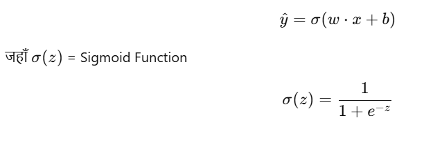
🎯 Prediction Function:


🎯 Decision Rule:

  • यदि y^0.5 → Class 1
  • अन्यथा → Class 0

🔧 उपयोग के क्षेत्र:

क्षेत्रउपयोग
Email FilterSpam vs Not Spam
हेल्थबीमारी है या नहीं
FinanceLoan Approve या Reject

🔬 Logistic Regression in PyTorch

import torch
import torch.nn as nn

# Dummy data for AND logic gate
X = torch.tensor([[0.,0.],[0.,1.],[1.,0.],[1.,1.]], dtype=torch.float32)
y = torch.tensor([[0.],[0.],[0.],[1.]], dtype=torch.float32)

# Logistic Regression Model
class LogisticRegression(nn.Module):
def __init__(self):
super().__init__()
self.linear = nn.Linear(2, 1)

def forward(self, x):
return torch.sigmoid(self.linear(x))

model = LogisticRegression()

# Loss and Optimizer
criterion = nn.BCELoss() # Binary Cross Entropy Loss
optimizer = torch.optim.SGD(model.parameters(), lr=0.1)

# Training
for epoch in range(1000):
y_pred = model(X)
loss = criterion(y_pred, y)
optimizer.zero_grad()
loss.backward()
optimizer.step()

if epoch % 100 == 0:
print(f"Epoch {epoch}, Loss: {loss.item():.4f}")

# Prediction
with torch.no_grad():
print("Prediction for [1, 1]:", model(torch.tensor([[1., 1.]])).item())

📊 Summary Table:

ElementDescription
TypeClassification
InputContinuous (Features)
OutputProbability (0 to 1)
ActivationSigmoid
Loss FunctionBinary Cross Entropy (BCELoss)
PyTorch Layernn.Linear() + torch.sigmoid()

Logistic Regression with Visualization (AND Gate)

import torch
import torch.nn as nn
import matplotlib.pyplot as plt
import numpy as np

# Dummy data (AND gate)
X = torch.tensor([[0.,0.],[0.,1.],[1.,0.],[1.,1.]], dtype=torch.float32)
y = torch.tensor([[0.],[0.],[0.],[1.]], dtype=torch.float32)

# Logistic Regression Model
class LogisticRegression(nn.Module):
def __init__(self):
super().__init__()
self.linear = nn.Linear(2, 1)

def forward(self, x):
return torch.sigmoid(self.linear(x))

model = LogisticRegression()
criterion = nn.BCELoss()
optimizer = torch.optim.SGD(model.parameters(), lr=0.1)

# Training
for epoch in range(1000):
y_pred = model(X)
loss = criterion(y_pred, y)
optimizer.zero_grad()
loss.backward()
optimizer.step()

if epoch % 100 == 0:
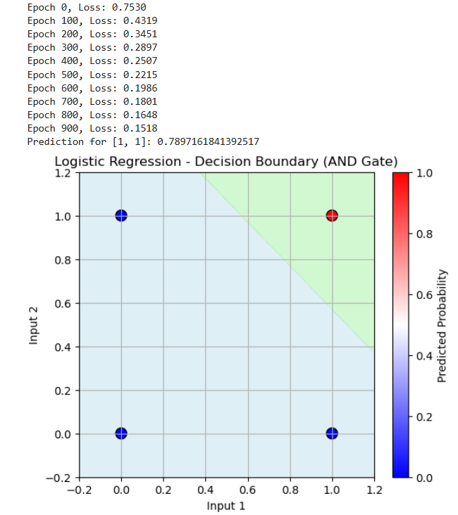
print(f"Epoch {epoch}, Loss: {loss.item():.4f}")

# Prediction test
with torch.no_grad():
test_input = torch.tensor([[1., 1.]])
pred = model(test_input)
print("Prediction for [1, 1]:", pred.item())

# ✅ Visualization Code Starts Here

# Convert to numpy for plotting
X_np = X.numpy()
y_np = y.numpy()

# Create a mesh grid
xx, yy = np.meshgrid(np.linspace(-0.2, 1.2, 100), np.linspace(-0.2, 1.2, 100))
grid = torch.tensor(np.c_[xx.ravel(), yy.ravel()], dtype=torch.float32)

with torch.no_grad():
probs = model(grid).reshape(xx.shape)

# Plot decision boundary
plt.figure(figsize=(6,5))
plt.contourf(xx, yy, probs, levels=[0, 0.5, 1], alpha=0.4, colors=['lightblue','lightgreen'])
plt.scatter(X_np[:,0], X_np[:,1], c=y_np[:,0], cmap='bwr', edgecolor='k', s=100)
plt.title("Logistic Regression - Decision Boundary (AND Gate)")
plt.xlabel("Input 1")
plt.ylabel("Input 2")
plt.colorbar(label='Predicted Probability')
plt.grid(True)
plt.show()

Output:

📝 Practice Questions:

  1. Logistic Regression को Classification के लिए क्यों उपयोग करते हैं?
  2. Sigmoid Function का role क्या होता है?
  3. Linear Regression और Logistic Regression में क्या मुख्य अंतर है?
  4. Binary Cross Entropy Loss क्या होता है?
  5. PyTorch में model.parameters() का क्या उपयोग है?

Linear Regression


🔷 परिचय:

Linear Regression सबसे सरल और प्रचलित Supervised Learning algorithm है।
इसका उद्देश्य है — किसी continuous value को predict करना, जैसे:

  • घर की कीमत
  • स्टूडेंट के मार्क्स
  • कर्मचारी का वेतन

🔶 फॉर्मूला:

🎯 Prediction Function:

जहाँ:

  • x= इनपुट
  • w = वज़न (weight)
  • b = बायस (bias)
  • y^ = अनुमानित आउटपुट (predicted output)

🔧 उपयोग:

क्षेत्रउदाहरण
रियल एस्टेटघर की कीमत का पूर्वानुमान
एजुकेशनमार्क्स का अनुमान
हेल्थरोग की गंभीरता स्कोर

🔢 Cost Function (Loss):

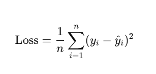
Mean Squared Error (MSE):


🔬 Linear Regression in PyTorch

import torch
import torch.nn as nn
import matplotlib.pyplot as plt

# Dummy dataset
X = torch.tensor([[1.0], [2.0], [3.0], [4.0]], dtype=torch.float32)
y = torch.tensor([[2.0], [4.0], [6.0], [8.0]], dtype=torch.float32)

# Linear Regression Model
model = nn.Linear(1, 1)

# Loss and Optimizer
criterion = nn.MSELoss()
optimizer = torch.optim.SGD(model.parameters(), lr=0.01)

# Training loop
epochs = 1000
for epoch in range(epochs):
y_pred = model(X)
loss = criterion(y_pred, y)
optimizer.zero_grad()
loss.backward()
optimizer.step()

if epoch % 100 == 0:
print(f'Epoch {epoch}, Loss: {loss.item():.4f}')

# Prediction
with torch.no_grad():
test = torch.tensor([[5.0]])
pred = model(test)
print("Prediction for 5.0:", pred.item())

# Visualize
predicted = model(X).detach()
plt.scatter(X, y, label='Original')
plt.plot(X, predicted, label='Fitted line', color='red')
plt.legend()
plt.show()

📊 Summary Table:

ElementDescription
Model TypeRegression
InputContinuous/Real number
OutputContinuous value
Loss FunctionMean Squared Error (MSE)
OptimizerSGD, Adam
Library UsedPyTorch

📝 Practice Questions:

  1. Linear Regression का उद्देश्य क्या होता है?
  2. Model का फॉर्मूला y^=w⋅x+b का मतलब समझाइए।
  3. MSE (Mean Squared Error) को क्यों उपयोग करते हैं?
  4. PyTorch में nn.Linear() क्या करता है?
  5. Optimizer का कार्य क्या होता है?

Introduction of Supervised Learning Algorithms

Supervised Learning वह तकनीक है जिसमें मॉडल को ऐसे डेटा पर प्रशिक्षित किया जाता है जिसमें इनपुट के साथ-साथ सही आउटपुट (label) भी होता है।
उदाहरण:

Input (Features)Output (Label)
उम्र = 30, वेतन = ₹40kलोन स्वीकृत (Yes)

अब हम ऐसे प्रमुख एल्गोरिद्म्स को समझेंगे जो Supervised Learning में सबसे ज़्यादा उपयोग होते हैं।


🔷 🔹 Why Supervised Algorithms?

FeatureBenefit
Input-output mapping definedआसानी से train और evaluate किया जा सकता है
Classification & Regression दोनों के लिएबहुत versatile models उपलब्ध हैं
Scalabilityछोटे से बड़े डेटासेट तक लागू होता है

🔶 Supervised Learning Algorithms के दो प्रमुख प्रकार:

प्रकारउपयोग क्षेत्रउदाहरण
ClassificationLabel पहचाननाEmail Spam, Disease Detection
RegressionValue predict करनाHouse Price, Stock Prediction

🔷 1. Linear Regression (रेखीय प्रतिगमन)

📌 उपयोग:

Continuous Value Prediction
(जैसे घर की कीमत, तापमान)

🧮 फॉर्मूला:

y = w*x + b

✅ Python Example:

from sklearn.linear_model import LinearRegression

model = LinearRegression()
model.fit(X_train, y_train)
y_pred = model.predict(X_test)

🔷 2. Logistic Regression (तर्कशक्ति प्रतिगमन)

📌 उपयोग:

Binary Classification (Yes/No)

✅ Output:

Probability (0 to 1), फिर threshold लगाकर decision

from sklearn.linear_model import LogisticRegression

model = LogisticRegression()
model.fit(X_train, y_train)
y_pred = model.predict(X_test)

🔷 3. Decision Tree

📌 उपयोग:

Classification और Regression दोनों के लिए
डाटा को बार-बार विभाजित करके निर्णय लेना।

from sklearn.tree import DecisionTreeClassifier

model = DecisionTreeClassifier()
model.fit(X_train, y_train)

🔷 4. Random Forest

📌 क्या है?

Multiple Decision Trees का ensemble
Voting या averaging के ज़रिए output देता है।

from sklearn.ensemble import RandomForestClassifier

model = RandomForestClassifier(n_estimators=100)
model.fit(X_train, y_train)

🔷 5. Support Vector Machine (SVM)

📌 उपयोग:

High-dimensional datasets में classification के लिए बेहतरीन

from sklearn.svm import SVC

model = SVC(kernel='linear')
model.fit(X_train, y_train)

🔷 6. K-Nearest Neighbors (KNN)

📌 उपयोग:

Instance-based learning — training में कोई model नहीं, prediction के समय नज़दीकी K-पड़ोसियों को देखता है।

from sklearn.neighbors import KNeighborsClassifier

model = KNeighborsClassifier(n_neighbors=3)
model.fit(X_train, y_train)

🔷 7. Naive Bayes

📌 उपयोग:

Text classification जैसे spam detection
(Statistical probability आधारित)

from sklearn.naive_bayes import GaussianNB

model = GaussianNB()
model.fit(X_train, y_train)

📊 Summary Table:

AlgorithmTypeStrengthsUse Case
Linear RegressionRegressionSimple, fastPrice prediction
Logistic RegressionClassificationProbabilistic outputSpam detection
Decision TreeBothInterpretabilityCredit approval
Random ForestBothAccuracy, handles overfittingMedical diagnosis
SVMClassificationWorks in high dimensionsFace recognition
KNNClassificationNo training, easy to implementPattern recognition
Naive BayesClassificationFast, good for textSentiment analysis

📝 Practice Questions:

  1. Linear Regression और Logistic Regression में क्या अंतर है?
  2. Random Forest को Decision Tree से बेहतर क्यों माना जाता है?
  3. SVM किस तरह से Classification करता है?
  4. KNN में K का चुनाव कैसे किया जाता है?
  5. Naive Bayes कब अच्छा और कब बेकार perform करता है?

Feature Selection & Feature Extraction

मशीन लर्निंग में सही फीचर्स (गुण) चुनना और नए उपयोगी फीचर्स बनाना मॉडल की दक्षता और सटीकता को कई गुना बढ़ा सकता है। यह प्रक्रिया दो भागों में बाँटी जाती है:
🔹 Feature Selection (चयन)
🔹 Feature Extraction (नव-निर्माण)


🔷 Why Feature Selection & Extraction?

ReasonBenefit
Less ComplexityModel simple और fast होता है
Overfitting से बचावUnnecessary features हटाने से accuracy बढ़ती है
Better PerformanceRelevant features रखने से result अच्छा आता है
Visualization आसान होती हैDimensionality घटाने से data समझना आसान होता है

🔶 1. Feature Selection (फीचर चयन)

📌 क्या है?

डेटा में से सबसे ज़रूरी और उपयोगी फीचर्स को चुनना, बाकी को हटाना। इससे model तेज़, सटीक और आसान बनता है।

✅ मुख्य तरीके:

तरीकाविवरण
Filter MethodsStatistics जैसे correlation, chi-square आदि के आधार पर फीचर्स चुनना
Wrapper Methodsहर फीचर सेट पर मॉडल train करके best चुनना (जैसे RFE)
Embedded Methodsमॉडल खुद feature चुनता है (जैसे Lasso, Decision Trees)

🛠️ Python Code Example (Correlation Method):

import pandas as pd
import seaborn as sns
import matplotlib.pyplot as plt

# Correlation Matrix
corr = df.corr()
sns.heatmap(corr, annot=True, cmap='coolwarm')
plt.show()

🔶 2. Feature Extraction (फीचर नव-निर्माण)

📌 क्या है?

मौजूदा फीचर्स से नए meaningful फीचर्स बनाना, या features को lower dimensions में compress करना।

उदाहरण:
Image data → Raw pixels को CNN features में बदला जाता है
Text data → TF-IDF या Word Embedding बनाया जाता है


✅ मुख्य तरीके:

तरीकाविवरण
PCA (Principal Component Analysis)Variance-preserving compressed representation
LDA (Linear Discriminant Analysis)Class separation के लिए feature reduce
AutoencodersDeep Learning आधारित compressed features
TF-IDF / Word2VecText से semantic features बनाना

🛠️ Python Code Example (PCA):

from sklearn.decomposition import PCA
from sklearn.preprocessing import StandardScaler

# Step 1: Scaling
scaler = StandardScaler()
X_scaled = scaler.fit_transform(df)

# Step 2: Apply PCA
pca = PCA(n_components=2)
X_pca = pca.fit_transform(X_scaled)

print("Reduced Features:\n", X_pca)

🔍 Feature Selection vs Feature Extraction

ComparisonFeature SelectionFeature Extraction
उद्देश्यसबसे अच्छे मौजूदा फीचर्स चुननानए meaningful फीचर्स बनाना
Feature Countकम होता हैअलग set of features बनते हैं
Technique ExamplesCorrelation, RFE, LassoPCA, Autoencoders, Word2Vec
व्याख्या आसान हैहाँकभी-कभी नहीं (PCA जैसे में)

📊 Summary Table:

TaskTool/Technique
SelectionCorrelation, Chi-square, RFE
EmbeddedLasso, Decision Tree
ExtractionPCA, LDA, Autoencoder
Text ExtractionTF-IDF, Word2Vec, BERT

📝 Practice Questions:

  1. Feature Selection और Feature Extraction में क्या अंतर है?
  2. PCA का क्या उपयोग है और कब किया जाता है?
  3. Wrapper method और Filter method में क्या फ़र्क है?
  4. Autoencoder का उपयोग feature extraction में कैसे होता है?
  5. Embedded Method का उदाहरण दीजिए।